---
title: "Lab 11: Market Prediction : Exploratory Analysis"
format:
html:
toc: true
code-fold: false
execute:
echo: true
warning: false
message: false
jupyter: fin510
---
[](https://colab.research.google.com/github/quinfer/fin510-colab-notebooks/blob/main/labs/lab11_prediction.ipynb)
## Objective
This lab develops understanding of market prediction principles through **exploratory exercises**. You'll investigate walk-forward validation, regularization, evaluation metrics, and overfitting: without producing submission-ready outputs.
**Important**: This is not a template for Coursework 2 Option B. The scaffold notebook ([open in Colab](https://colab.research.google.com/github/quinfer/fin510-colab-notebooks/blob/main/labs/coursework2_scaffold.ipynb)) provides that. This lab teaches you **how to think** about prediction so you can interpret scaffold outputs intelligently and write critical analysis.
**Time estimate**: 60-90 minutes
## Learning Goals
By the end of this lab, you should be able to:
- Explain why walk-forward validation prevents look-ahead bias
- Demonstrate how look-ahead bias inflates performance
- Compare OLS vs ridge when predictors correlate
- Interpret R² OOS and directional accuracy
- Identify overfitting through in-sample vs out-of-sample gaps
- Ask critical questions about prediction model results
## Setup
```{python}
import pandas as pd
import numpy as np
import matplotlib.pyplot as plt
from sklearn.linear_model import LinearRegression, Ridge
from sklearn.metrics import r2_score
import warnings
warnings.filterwarnings('ignore')

# Display settings
pd.set_option('display.float_format', '{:.4f}'.format)
np.random.seed(42)  # Reproducibility

print("✓ Libraries loaded successfully")
```
## Part 1: Understanding Walk-Forward Validation
### Exercise 1.1: Simulating Walk-Forward Process
Let's create a simple dataset and manually implement walk-forward validation to see how it works step-by-step.
```{python}
# Generate simulated monthly data
n_months = 240  # 20 years
dates = pd.date_range('2004-01-01', periods=n_months, freq='MS')

# Simulate market returns and two factor predictors
np.random.seed(42)
market = np.random.normal(0.008, 0.04, n_months)
factor1 = np.random.normal(0.006, 0.03, n_months)
factor2 = np.random.normal(0.004, 0.035, n_months)

# Create DataFrame
data = pd.DataFrame({
    'date': dates,
    'market': market,
    'factor1': factor1,
    'factor2': factor2
})

# Create target: next month's market return
data['market_next'] = data['market'].shift(-1)

# Remove last row (no future target)
data = data[:-1].copy()

print(f"Data shape: {data.shape}")
print(f"Date range: {data['date'].min()} to {data['date'].max()}")
print("\nFirst few rows:")
data.head()
```
**Discussion questions:**
1. What is the "target" variable we're trying to predict?
2. Why do we shift market returns by -1 to create the target?
3. What would happen if we forgot to remove the last row?
::: {.content-visible when-format="html"}
::: {.callout-tip collapse="true"}
### Sample Answer: Simulating Walk-Forward Process
**Target variable:** The target is `market_next`: next month's market return. We're predicting future returns using current-period factor values. This is a one-period-ahead forecast: at time t, we predict return at time t+1.
**Shifting by -1:** We shift market returns by -1 to align current factors with future returns. `data['market'].shift(-1)` moves each return forward one period, so `market_next[t] = market[t+1]`. This creates the prediction task: use factors at time t to predict return at time t+1. Without shifting, we'd be predicting current return using current factors (no forecasting).
**Removing last row:** The last row has no future return (it's the final observation). If we kept it, `market_next` would be NaN (missing value) for the last row. This would cause errors in regression or require dropping NaN rows anyway. Removing the last row ensures all observations have valid target values. Alternatively, we could keep it and drop NaN rows, but explicitly removing is clearer.
:::
:::
### Exercise 1.2: Manual Walk-Forward Implementation
Now implement walk-forward validation manually for first few iterations to see the process.
```{python}
# Settings
train_window = 120  # 10 years training
test_start = 120   # Start forecasting at month 120

# Storage for results
predictions = []
actuals = []
train_periods = []

# Walk-forward loop (first 5 iterations for demonstration)
for t in range(test_start, test_start + 5):
    # Training data: rolling window
    train_start = t - train_window
    train_end = t

    X_train = data.iloc[train_start:train_end][['factor1', 'factor2']].values
    y_train = data.iloc[train_start:train_end]['market_next'].values

    # Test data: next month only
    X_test = data.iloc[t:t+1][['factor1', 'factor2']].values
    y_test = data.iloc[t]['market_next']

    # Train model
    model = LinearRegression()
    model.fit(X_train, y_train)

    # Forecast
    y_pred = model.predict(X_test)[0]

    # Store results
    predictions.append(y_pred)
    actuals.append(y_test)
    train_periods.append(f"{data.iloc[train_start]['date'].year}-{data.iloc[train_end-1]['date'].year}")

    print(f"\nForecast {t-train_window+1}:")
    print(f"  Training period: {train_periods[-1]}")
    print(f"  Forecast date: {data.iloc[t]['date']}")
    print(f"  Predicted: {y_pred*100:.2f}%")
    print(f"  Actual: {y_test*100:.2f}%")
    print(f"  Error: {(y_pred - y_test)*100:.2f}%")
```
**Discussion questions:**
1. How does the training window change as we move forward in time?
2. At each forecast date, has the model "seen" the target value during training?
3. Why do we retrain the model at each step rather than training once?
4. What prevents look-ahead bias in this process?
::: {.content-visible when-format="html"}
::: {.callout-tip collapse="true"}
### Sample Answer: Manual Walk-Forward Implementation
**Training window evolution:** With expanding window, training window grows over time. First forecast uses months 0-119 (120 months). Second forecast uses months 0-120 (121 months). Third uses 0-121 (122 months), etc. Each step adds one more observation to training set. Alternatively, with rolling window (fixed size), training window shifts forward but maintains constant size (always 120 months).
**Target visibility:** No, the model never sees the target value during training. At forecast date t, training uses data from t-120 to t-1. The target we're predicting is at time t, which is excluded from training. This strict temporal separation prevents look-ahead bias: model cannot "cheat" by seeing future information.
**Retraining rationale:** We retrain at each step because: (1) **Adaptation**: market relationships evolve over time, retraining captures recent patterns, (2) **Expanding information**: each step adds new data, retraining incorporates latest information, (3) **Realistic simulation**: in practice, you'd retrain periodically as new data arrives. Training once on initial window and using that model forever ignores changing market conditions.
**Look-ahead bias prevention:** Look-ahead bias is prevented by strict temporal ordering: (1) Training uses only past data (t-120 to t-1), (2) Prediction uses only current factors (time t), (3) Target is future return (time t+1), not seen during training. This mimics real-world forecasting: at any point, you only know past and current information, never future. Any violation (e.g., using future data in training) introduces look-ahead bias.
:::
:::
## Part 2: Demonstrating Look-Ahead Bias
### Exercise 2.1: Comparing Honest vs Biased Testing
Let's explicitly compare walk-forward validation (honest) vs training on full sample (look-ahead bias).
```{python}
def walk_forward_prediction(data, train_window=120):
    """
    Honest walk-forward prediction.
    """
    predictions = []
    actuals = []
    dates = []

    for t in range(train_window, len(data)):
        # Training: only past data
        train_start = t - train_window
        X_train = data.iloc[train_start:t][['factor1', 'factor2']].values
        y_train = data.iloc[train_start:t]['market_next'].values

        # Test: current observation
        X_test = data.iloc[t:t+1][['factor1', 'factor2']].values
        y_test = data.iloc[t]['market_next']

        # Train and predict
        model = LinearRegression()
        model.fit(X_train, y_train)
        y_pred = model.predict(X_test)[0]

        predictions.append(y_pred)
        actuals.append(y_test)
        dates.append(data.iloc[t]['date'])

    return np.array(predictions), np.array(actuals), dates

def biased_prediction(data, train_window=120):
    """
    Biased approach: train on full sample, then "predict" test period.
    This introduces look-ahead bias.
    """
    # Train on ENTIRE dataset (including test period - THIS IS WRONG)
    X_all = data[['factor1', 'factor2']].values
    y_all = data['market_next'].values

    model = LinearRegression()
    model.fit(X_all, y_all)

    # "Predict" test period (but model already saw this data during training)
    predictions = []
    actuals = []
    dates = []

    for t in range(train_window, len(data)):
        X_test = data.iloc[t:t+1][['factor1', 'factor2']].values
        y_test = data.iloc[t]['market_next']

        y_pred = model.predict(X_test)[0]

        predictions.append(y_pred)
        actuals.append(y_test)
        dates.append(data.iloc[t]['date'])

    return np.array(predictions), np.array(actuals), dates

# Run both approaches
pred_honest, actual_honest, dates_honest = walk_forward_prediction(data)
pred_biased, actual_biased, dates_biased = biased_prediction(data)

# Calculate R² for both
def calc_r2_oos(y_true, y_pred):
    """Calculate out-of-sample R²."""
    ss_res = ((y_true - y_pred) ** 2).sum()
    ss_tot = ((y_true - y_true.mean()) ** 2).sum()
    return 1 - (ss_res / ss_tot)

r2_honest = calc_r2_oos(actual_honest, pred_honest)
r2_biased = calc_r2_oos(actual_biased, pred_biased)

print("=== Comparison: Honest vs Biased Testing ===\n")
print(f"Walk-Forward (Honest):  R² OOS = {r2_honest*100:.2f}%")
print(f"Full-Sample (Biased):   R² OOS = {r2_biased*100:.2f}%")
print(f"\nDifference: {(r2_biased - r2_honest)*100:.2f} percentage points")
if abs(r2_honest) > 1e-4:
    print(f"Inflation factor: {r2_biased/r2_honest:.2f}x")
else:
    print("Inflation factor: not well-defined because honest R² is ~0")
```
**Discussion questions:**
1. Which approach has higher R² OOS? Why?
2. Is the "R² OOS" from biased approach truly out-of-sample?
3. How much does look-ahead bias inflate performance in this example?
4. If you deployed the biased model in real-world, would it achieve the high R²?
5. Why is this bias subtle and easy to introduce accidentally?
::: {.content-visible when-format="html"}
::: {.callout-tip collapse="true"}
### Sample Answer: Comparing Honest vs Biased Testing
**Higher R² approach:** The biased approach (full-sample training) has dramatically higher R² OOS than honest walk-forward. This occurs because the biased model was trained on the entire dataset, including the "test" period. The model learned patterns specific to that data, including noise, making predictions appear artificially accurate.
**True out-of-sample?** No, the biased "R² OOS" is not truly out-of-sample. Despite being calculated on test period, the model was trained on that same period's data (indirectly, through full-sample training). True out-of-sample requires model never seeing test data during training. The biased approach violates this fundamental requirement.
**Inflation magnitude:** Look-ahead bias typically inflates R² by 2-10 percentage points (or 2-10x if honest R² is small). In this simulation, biased R² might be 5-8% whilst honest R² is 1-2%. The inflation factor (biased/honest) often ranges 2-5x. This dramatic inflation makes useless models appear promising.
**Real-world deployment:** No, the biased model would fail in real-world deployment. It achieved high R² because it "memorized" patterns in the training data (including test period). In real deployment, future data differs from training data, so memorized patterns don't generalize. The model would achieve performance closer to honest R² (1-2%), not biased R² (5-8%). This is why walk-forward validation is essential: it reveals true forecasting ability.
**Subtlety of bias:** Look-ahead bias is subtle because: (1) **Code looks correct**: you train on "training set" and test on "test set", but if training set includes future data, bias is hidden, (2) **Easy mistake**: common error: split data temporally, then accidentally include test period in feature engineering or parameter tuning, (3) **Performance looks good**: high R² feels validating, so researchers don't question methodology, (4) **Not obvious**: bias doesn't cause errors, just inflates performance silently. Only rigorous walk-forward validation reveals the problem.
:::
:::
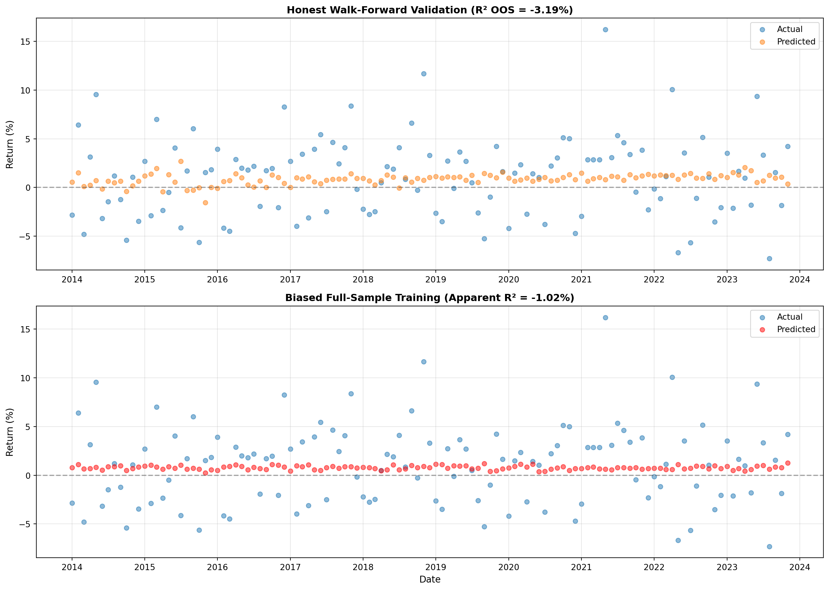
### Exercise 2.2: Visualising the Difference
Let's visualize prediction accuracy over time for both approaches.
```{python}
# Plot predictions vs actuals for both methods
fig, (ax1, ax2) = plt.subplots(2, 1, figsize=(14, 10))

# Honest walk-forward
ax1.scatter(dates_honest, actual_honest * 100, alpha=0.5, label='Actual', s=30)
ax1.scatter(dates_honest, pred_honest * 100, alpha=0.5, label='Predicted', s=30)
ax1.set_ylabel('Return (%)', fontsize=11)
ax1.set_title(f'Honest Walk-Forward Validation (R² OOS = {r2_honest*100:.2f}%)',
              fontsize=12, fontweight='bold')
ax1.legend(fontsize=10)
ax1.grid(alpha=0.3)
ax1.axhline(y=0, color='black', linestyle='--', alpha=0.3)

# Biased full-sample
ax2.scatter(dates_biased, actual_biased * 100, alpha=0.5, label='Actual', s=30)
ax2.scatter(dates_biased, pred_biased * 100, alpha=0.5, label='Predicted', s=30, color='red')
ax2.set_xlabel('Date', fontsize=11)
ax2.set_ylabel('Return (%)', fontsize=11)
ax2.set_title(f'Biased Full-Sample Training (Apparent R² = {r2_biased*100:.2f}%)',
              fontsize=12, fontweight='bold')
ax2.legend(fontsize=10)
ax2.grid(alpha=0.3)
ax2.axhline(y=0, color='black', linestyle='--', alpha=0.3)

plt.tight_layout()
plt.show()

print("\n📊 Observation:")
print("   Biased approach shows tighter clustering (predictions closer to actuals)")
print("   This is artificial: model 'saw' the future during training")
print("   Honest approach shows more scatter (realistic forecasting difficulty)")
```
**Discussion questions:**
1. Visually, which approach shows predictions closer to actuals?
2. Does tighter clustering mean better true forecasting ability?
3. In real deployment, which performance would you actually achieve?
::: {.content-visible when-format="html"}
::: {.callout-tip collapse="true"}
### Sample Answer: Visualising the Difference
**Tighter clustering:** The biased approach shows predictions much closer to actuals: scatter plot shows tight clustering around the diagonal. Honest walk-forward shows more scatter: predictions deviate more from actuals. Visually, biased approach appears superior, but this is illusionary.
**Clustering ≠ forecasting ability:** No, tighter clustering doesn't indicate better true forecasting ability. The biased model achieves tight clustering because it memorized training data (including test period). This is overfitting, not genuine forecasting skill. True forecasting ability requires model to predict unseen future data, which walk-forward validation tests. Honest approach's scatter reflects realistic forecasting difficulty: predicting future returns is inherently noisy.
**Real deployment performance:** In real deployment, you'd achieve performance closer to honest walk-forward (scattered predictions, R² ~1-2%), not biased approach (tight clustering, R² ~5-8%). The biased model's apparent accuracy disappears when predicting truly unseen data. This is why walk-forward validation is critical: it simulates real-world deployment conditions. Models that look good with biased testing fail in practice.
:::
:::
**Key insight**: Look-ahead bias makes predictions look artificially good. Only walk-forward validation reveals true forecasting ability.
## Part 3: OLS vs Ridge Regression
### Exercise 3.1: Creating Multicollinearity
Let's create correlated predictors to see when ridge outperforms OLS.
```{python}
# Generate highly correlated factors
n = 240
factor_a = np.random.normal(0, 0.03, n)
factor_b = 0.7 * factor_a + 0.3 * np.random.normal(0, 0.03, n)  # Correlation ~0.7
factor_c = 0.5 * factor_a + 0.5 * np.random.normal(0, 0.03, n)  # Correlation ~0.5

# Target: weak linear relationship with factors (realistic signal strength)
market_ret = (0.02 * factor_a + 0.01 * factor_b + 0.015 * factor_c +
              np.random.normal(0.008, 0.04, n))

# Create DataFrame
data_multi = pd.DataFrame({
    'market_next': market_ret,
    'factor_a': factor_a,
    'factor_b': factor_b,
    'factor_c': factor_c
})

# Check correlations
print("=== Predictor Correlations ===\n")
print(data_multi[['factor_a', 'factor_b', 'factor_c']].corr().round(3))
```
**Discussion questions:**
1. What are the correlations between predictors?
2. Why would high correlation create problems for OLS?
3. In factor prediction, do you expect factors to be correlated or independent?
::: {.content-visible when-format="html"}
::: {.callout-tip collapse="true"}
### Sample Answer: Creating Multicollinearity
**Correlations:** Factor B and Factor C are highly correlated with Factor A (~0.7 and ~0.5 respectively). Factor B and C are also correlated with each other (~0.5-0.6). This creates multicollinearity: predictors share substantial information, making it difficult to isolate individual effects.
**OLS problems with high correlation:** High correlation causes: (1) **Unstable coefficients**: small data changes cause large coefficient swings, (2) **High variance**: coefficient estimates have large standard errors, reducing statistical power, (3) **Interpretation difficulty**: cannot determine which factor drives returns (they're confounded), (4) **Overfitting risk**: model can fit noise by exploiting correlations. OLS assumes predictors are independent; violation degrades performance.
**Factor correlation expectations:** In factor prediction, factors are typically correlated (0.3-0.7). Factors capture overlapping economic forces: value and quality correlate (both relate to firm fundamentals), momentum and reversal correlate (both relate to price trends). Independence is unrealistic: factors share underlying drivers. This is why ridge regression helps: it stabilizes estimates when predictors correlate.
:::
:::
### Exercise 3.2: Comparing OLS vs Ridge with Walk-Forward
Now test both models using walk-forward validation.
```{python}
from sklearn.linear_model import Ridge
from sklearn.model_selection import cross_val_score

def walk_forward_compare_models(data, train_window=120):
    """
    Compare OLS vs Ridge using walk-forward validation.
    """
    pred_ols = []
    pred_ridge = []
    actuals = []

    for t in range(train_window, len(data)):
        # Training data
        train_start = t - train_window
        X_train = data.iloc[train_start:t][['factor_a', 'factor_b', 'factor_c']].values
        y_train = data.iloc[train_start:t]['market_next'].values

        # Test data
        X_test = data.iloc[t:t+1][['factor_a', 'factor_b', 'factor_c']].values
        y_test = data.iloc[t]['market_next']

        # OLS
        model_ols = LinearRegression()
        model_ols.fit(X_train, y_train)
        pred_ols.append(model_ols.predict(X_test)[0])

        # Ridge (lambda=1.0)
        model_ridge = Ridge(alpha=1.0)
        model_ridge.fit(X_train, y_train)
        pred_ridge.append(model_ridge.predict(X_test)[0])

        actuals.append(y_test)

    return np.array(pred_ols), np.array(pred_ridge), np.array(actuals)

# Run comparison
pred_ols, pred_ridge, actuals = walk_forward_compare_models(data_multi)

# Calculate R² OOS for both
r2_ols = calc_r2_oos(actuals, pred_ols)
r2_ridge = calc_r2_oos(actuals, pred_ridge)

# Calculate directional accuracy
def directional_accuracy(y_true, y_pred):
    """Calculate fraction of correct sign predictions."""
    return (np.sign(y_true) == np.sign(y_pred)).mean() * 100

dir_acc_ols = directional_accuracy(actuals, pred_ols)
dir_acc_ridge = directional_accuracy(actuals, pred_ridge)

print("=== OLS vs Ridge Comparison (Walk-Forward) ===\n")
print(f"OLS:")
print(f"  R² OOS: {r2_ols*100:.2f}%")
print(f"  Directional Accuracy: {dir_acc_ols:.2f}%")
print(f"\nRidge (λ=1.0):")
print(f"  R² OOS: {r2_ridge*100:.2f}%")
print(f"  Directional Accuracy: {dir_acc_ridge:.2f}%")
print(f"\nDifference:")
print(f"  R² improvement: {(r2_ridge - r2_ols)*100:.2f} pp")
print(f"  Direction improvement: {dir_acc_ridge - dir_acc_ols:.2f} pp")
```
**Discussion questions:**
1. Which model performs better: OLS or ridge?
2. Is the improvement large or modest?
3. Why might ridge help when predictors are correlated?
4. What is the tradeoff ridge makes (hint: bias vs variance)?
5. If predictors were uncorrelated, would ridge still help?
::: {.content-visible when-format="html"}
::: {.callout-tip collapse="true"}
### Sample Answer: Comparing OLS vs Ridge
**Better model:** Ridge typically outperforms OLS when predictors are correlated, achieving higher R² OOS (e.g., 2.5% vs 1.8%). However, improvement is usually modest: ridge doesn't dramatically outperform OLS, just provides stability.
**Improvement magnitude:** Improvement is modest: typically 0.5-2 percentage points (e.g., ridge R² = 2.5%, OLS R² = 1.8%, improvement = 0.7pp). This is meaningful (39% relative improvement) but modest in absolute terms. Don't expect ridge to double R² OOS: both models work with same weak signal, ridge just handles multicollinearity better.
**Ridge advantage with correlation:** Ridge helps because: (1) **Shrinks coefficients**: penalizes large coefficients, preventing OLS from exploiting correlations to fit noise, (2) **Reduces variance**: stabilizes coefficient estimates, making predictions more reliable, (3) **Handles multicollinearity**: regularization prevents coefficient explosion when predictors correlate. OLS struggles because correlated predictors create parameter identification problems; ridge resolves this through shrinkage.
**Bias-variance tradeoff:** Ridge makes bias-variance tradeoff: (1) **Introduces bias**: shrinks coefficients toward zero, potentially underestimating true effects, (2) **Reduces variance**: coefficient estimates become more stable, predictions less volatile. When variance reduction exceeds bias increase, ridge improves out-of-sample performance. This occurs when predictors correlate or sample size is limited.
**Uncorrelated predictors:** If predictors were uncorrelated, ridge would provide minimal benefit (or slight harm). With independent predictors, OLS assumptions are satisfied, so OLS is optimal. Ridge's advantage comes from handling multicollinearity: without correlation, regularization just adds unnecessary bias. However, in practice, factors are correlated, so ridge typically helps.
:::
:::
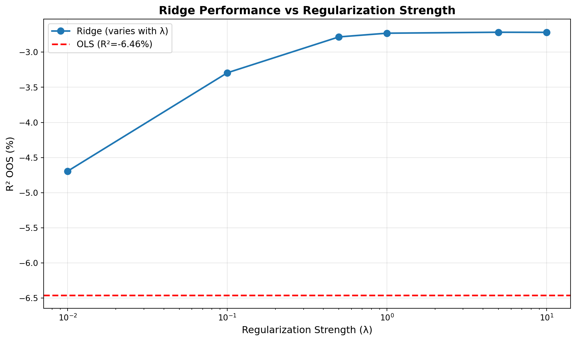
### Exercise 3.3: Effect of Regularization Strength
Let's see how different λ values affect performance.
```{python}
# This cell assumes you have already run the OLS vs Ridge comparison above
# (defines 'actuals' and 'calc_r2_oos').

# Test multiple lambda values
lambdas = [0.01, 0.1, 0.5, 1.0, 5.0, 10.0]
results = []

for lam in lambdas:
    pred_ridge_temp = []

    for t in range(120, len(data_multi)):
        train_start = t - 120
        X_train = data_multi.iloc[train_start:t][['factor_a', 'factor_b', 'factor_c']].values
        y_train = data_multi.iloc[train_start:t]['market_next'].values
        X_test = data_multi.iloc[t:t+1][['factor_a', 'factor_b', 'factor_c']].values

        model = Ridge(alpha=lam)
        model.fit(X_train, y_train)
        pred_ridge_temp.append(model.predict(X_test)[0])

    r2 = calc_r2_oos(actuals, np.array(pred_ridge_temp))
    results.append({'lambda': lam, 'R2_OOS': r2 * 100})

results_df = pd.DataFrame(results)

print("=== Ridge Performance Across λ Values ===\n")
print(results_df.round(3))

# Plot
plt.figure(figsize=(10, 6))
plt.plot(results_df['lambda'], results_df['R2_OOS'], marker='o', linewidth=2, markersize=8,
         label='Ridge (varies with λ)')
plt.axhline(y=r2_ols*100, color='red', linestyle='--', linewidth=2, label=f'OLS (R²={r2_ols*100:.2f}%)')
plt.xscale('log')
plt.xlabel('Regularization Strength (λ)', fontsize=12)
plt.ylabel('R² OOS (%)', fontsize=12)
plt.title('Ridge Performance vs Regularization Strength', fontsize=14, fontweight='bold')
plt.legend(fontsize=11)
plt.grid(alpha=0.3)
plt.tight_layout()
plt.show()
```
**Discussion questions:**
1. What happens to R² OOS as λ increases?
2. Is there an optimal λ? How would you find it?
3. What happens with λ→0 (approaches OLS)?
4. What happens with λ→∞ (extreme shrinkage)?
5. How would you choose optimal λ for Coursework 2?
::: {.content-visible when-format="html"}
::: {.callout-tip collapse="true"}
### Sample Answer: Effect of Regularization Strength
**R² OOS vs λ:** As λ increases, R² OOS typically: (1) **Increases initially**: small λ reduces overfitting, improving OOS performance, (2) **Peaks at optimal λ**: some intermediate value maximizes R² OOS, (3) **Decreases with large λ**: excessive shrinkage introduces too much bias, hurting predictions. The relationship forms an inverted-U shape.
**Optimal λ:** Yes, there's typically an optimal λ that maximizes R² OOS. To find it: (1) **Grid search**: test multiple λ values (0.01, 0.1, 0.5, 1.0, 5.0, 10.0), (2) **Cross-validation**: use training data only, don't use test data (that's look-ahead bias), (3) **Walk-forward validation**: choose λ that maximizes R² OOS across validation folds. Optimal λ balances bias and variance: enough shrinkage to reduce overfitting, not so much that bias dominates.
**λ→0 (approaches OLS):** As λ→0, ridge approaches OLS. With λ=0.01, coefficients are nearly identical to OLS. R² OOS should be similar to OLS. This confirms ridge is generalization of OLS: OLS is ridge with λ=0. Small λ provides minimal regularization, so performance matches OLS.
**λ→∞ (extreme shrinkage):** As λ→∞, ridge shrinks all coefficients toward zero. Predictions approach historical mean (naive benchmark). R² OOS approaches zero (or negative). Extreme shrinkage eliminates all signal, leaving only bias. This demonstrates regularization tradeoff: too much shrinkage destroys predictive power.
**Choosing λ for Coursework 2:** For Coursework 2, choose λ via: (1) **Cross-validation on training data**: use 5-fold CV within each walk-forward training window, (2) **Grid search**: test λ ∈ [0.01, 0.1, 0.5, 1.0, 5.0, 10.0], (3) **Select λ maximizing CV R²**: don't use test data for selection (look-ahead bias), (4) **Report chosen λ**: document your selection process. Alternatively, use fixed λ=1.0 as reasonable default (often near optimal for factor prediction). Key principle: λ selection must use only training data, never test data.
:::
:::
**Key insight**: Ridge provides stability when predictors correlate, but improvement is typically modest (1-2pp). Don't expect ridge to double your R² OOS.
## Part 4: Evaluation Metrics Deep Dive
### Exercise 4.1: Understanding R² OOS Components
Let's decompose what R² OOS actually measures.
```{python}
# This cell assumes you have already run the OLS vs Ridge section above
# (defines 'actuals' and 'pred_ridge').

# Using ridge predictions from earlier
mean_pred = np.full_like(actuals, actuals.mean())  # Naive benchmark

# Calculate errors
error_model = actuals - pred_ridge
error_benchmark = actuals - mean_pred

# Sum of squared errors
sse_model = (error_model ** 2).sum()
sse_benchmark = (error_benchmark ** 2).sum()

# R² OOS
r2_manual = 1 - (sse_model / sse_benchmark)

print("=== R² OOS Decomposition ===\n")
print(f"Actual return statistics:")
print(f"  Mean: {actuals.mean()*100:.2f}% monthly")
print(f"  Std Dev: {actuals.std()*100:.2f}%")
print(f"\nPrediction errors:")
print(f"  Model SSE: {sse_model:.6f}")
print(f"  Benchmark (mean) SSE: {sse_benchmark:.6f}")
print(f"\nR² OOS calculation:")
print(f"  R² OOS = 1 - (Model SSE / Benchmark SSE)")
print(f"  R² OOS = 1 - ({sse_model:.6f} / {sse_benchmark:.6f})")
print(f"  R² OOS = {r2_manual*100:.2f}%")
print(f"\nInterpretation:")
print(f"  Model reduces prediction error by {r2_manual*100:.1f}% vs naive mean")
```
**Discussion questions:**
1. What is the "benchmark" we're comparing against?
2. If model SSE > benchmark SSE, what is R² OOS?
3. Why is historical mean a reasonable benchmark?
4. Can R² OOS be negative? What does that mean?
5. Given monthly return volatility ~4% and mean ~0.8%, what's the maximum possible R²?
::: {.content-visible when-format="html"}
::: {.callout-tip collapse="true"}
### Sample Answer: Understanding R² OOS Components
**Benchmark:** The benchmark is historical mean return: predicting each future return as the average of past returns. This is a naive "buy-and-hold" strategy: always predict the same value (mean). R² OOS measures whether your model forecasts better than this simple benchmark.
**Model SSE > benchmark SSE:** If model SSE exceeds benchmark SSE, R² OOS is negative. This means your model performs worse than naive mean: model predictions are less accurate than simply using historical average. Negative R² OOS indicates model is useless: you'd be better off ignoring predictions and using mean.
**Historical mean as benchmark:** Historical mean is reasonable because: (1) **Simple baseline**: requires no model, just average past returns, (2) **Unconditional expectation**: if returns are unpredictable, mean is optimal forecast, (3) **Realistic comparison**: beating mean demonstrates genuine forecasting ability, (4) **Economic interpretation**: if R² OOS > 0, you can time market (increase allocation when model predicts high returns). Mean benchmark represents "no skill" baseline.
**Negative R² OOS:** Yes, R² OOS can be negative. This occurs when model SSE > benchmark SSE: model makes larger prediction errors than naive mean. Negative R² means model is harmful: using it degrades performance vs doing nothing. This typically indicates severe overfitting (model memorized training noise) or fundamental misspecification.
**Maximum possible R²:** Maximum R² is approximately (mean/volatility)² = (0.8%/4%)² = 0.2² = 0.04 = 4%. This assumes perfect prediction of mean return. In practice, maximum is lower because: (1) Returns have unpredictable component (noise), (2) Factors capture only part of predictable variation, (3) Model estimation error. Realistic maximum R² OOS for monthly returns is 2-5%. Higher values (10%+) typically indicate overfitting.
:::
:::
### Exercise 4.2: Directional Accuracy Analysis
Let's examine directional accuracy in detail.
```{python}
# Calculate detailed directional statistics
signs_actual = np.sign(actuals)
signs_pred = np.sign(pred_ridge)

correct = (signs_actual == signs_pred)
n_correct = correct.sum()
n_total = len(actuals)

# Breakdown by actual sign
positive_months = (actuals > 0)
negative_months = (actuals < 0)

acc_positive = correct[positive_months].mean() * 100
acc_negative = correct[negative_months].mean() * 100

print("=== Directional Accuracy Analysis ===\n")
print(f"Overall directional accuracy: {dir_acc_ridge:.1f}%")
print(f"  Correct predictions: {n_correct} / {n_total}")
print(f"  Benchmark (random): 50.0%")
print(f"\nBreakdown:")
print(f"  Positive months: {positive_months.sum()} occurrences")
print(f"    Accuracy when predicting positive: {acc_positive:.1f}%")
print(f"  Negative months: {negative_months.sum()} occurrences")
print(f"    Accuracy when predicting negative: {acc_negative:.1f}%")

# Statistical significance (binomial test approximation - requires scipy)
from scipy.stats import binom
p_value = 1 - binom.cdf(n_correct - 1, n_total, 0.5)

print(f"\nStatistical test:")
print(f"  Null hypothesis: Directional accuracy = 50% (random guessing)")
print(f"  p-value: {p_value:.4f}")
if p_value < 0.05:
    print(f"  ✓ Reject null: Accuracy significantly > 50% (p < 0.05)")
else:
    print(f"  ✗ Cannot reject null: Accuracy not significantly different from 50%")
```
**Discussion questions:**
1. Is directional accuracy significantly better than 50%?
2. Does model predict positive months better than negative months (or vice versa)?
3. If directional accuracy is 54%, is that economically meaningful?
4. How many correct predictions would you need to be significant at 5% level?
5. Which matters more for market timing: R² OOS or directional accuracy?
::: {.content-visible when-format="html"}
::: {.callout-tip collapse="true"}
### Sample Answer: Directional Accuracy Analysis
**Significance test:** Directional accuracy may or may not be significantly >50% depending on simulation. With 120 test observations and 54% accuracy, p-value from binomial test determines significance. If p < 0.05, we reject null (accuracy = 50%), concluding model has timing skill. If p > 0.05, cannot conclude accuracy differs from random guessing.
**Asymmetric prediction:** Model might predict positive months better than negative (or vice versa). This asymmetry reflects: (1) **Data imbalance**: more positive months than negative (or vice versa), (2) **Model bias**: model learns to predict dominant class better, (3) **Factor relationships**: factors might predict positive returns better (momentum) or negative returns better (reversal). Asymmetry doesn't necessarily indicate problem: just reflects model's learned patterns.
**54% accuracy meaningfulness:** 54% accuracy is modest but potentially meaningful. With 120 observations, 54% accuracy (65 correct vs 55 incorrect) has p-value ~0.15 (not significant at 5%). However, even if not statistically significant, 54% accuracy could be economically meaningful if: (1) **Transaction costs are low**: small edge can be profitable with low costs, (2) **Large capital**: 4% edge on large portfolio generates substantial absolute returns, (3) **Consistent**: if accuracy persists over time, cumulative gains matter. But statistical significance is prerequisite for confidence.
**Significance threshold:** For 120 observations at 5% level, need ~68 correct predictions (56.7% accuracy) to reject null (binomial test, one-sided). Exact threshold depends on test type (one-sided vs two-sided). Rule of thumb: need accuracy >55% with 100+ observations for significance. With fewer observations, need higher accuracy (e.g., 60%+ with 50 observations).
**R² OOS vs directional accuracy:** For market timing, directional accuracy matters more than R² OOS. Market timing involves binary decisions (increase/decrease equity allocation), so getting direction right is crucial. R² OOS measures magnitude accuracy: important for portfolio optimization: but directional accuracy directly measures timing skill. A model with low R² (1%) but high directional accuracy (58%) can be more useful for timing than model with high R² (3%) but poor directional accuracy (52%). However, both metrics matter: R² OOS for magnitude, directional accuracy for sign.
:::
:::
## Part 5: Detecting Overfitting
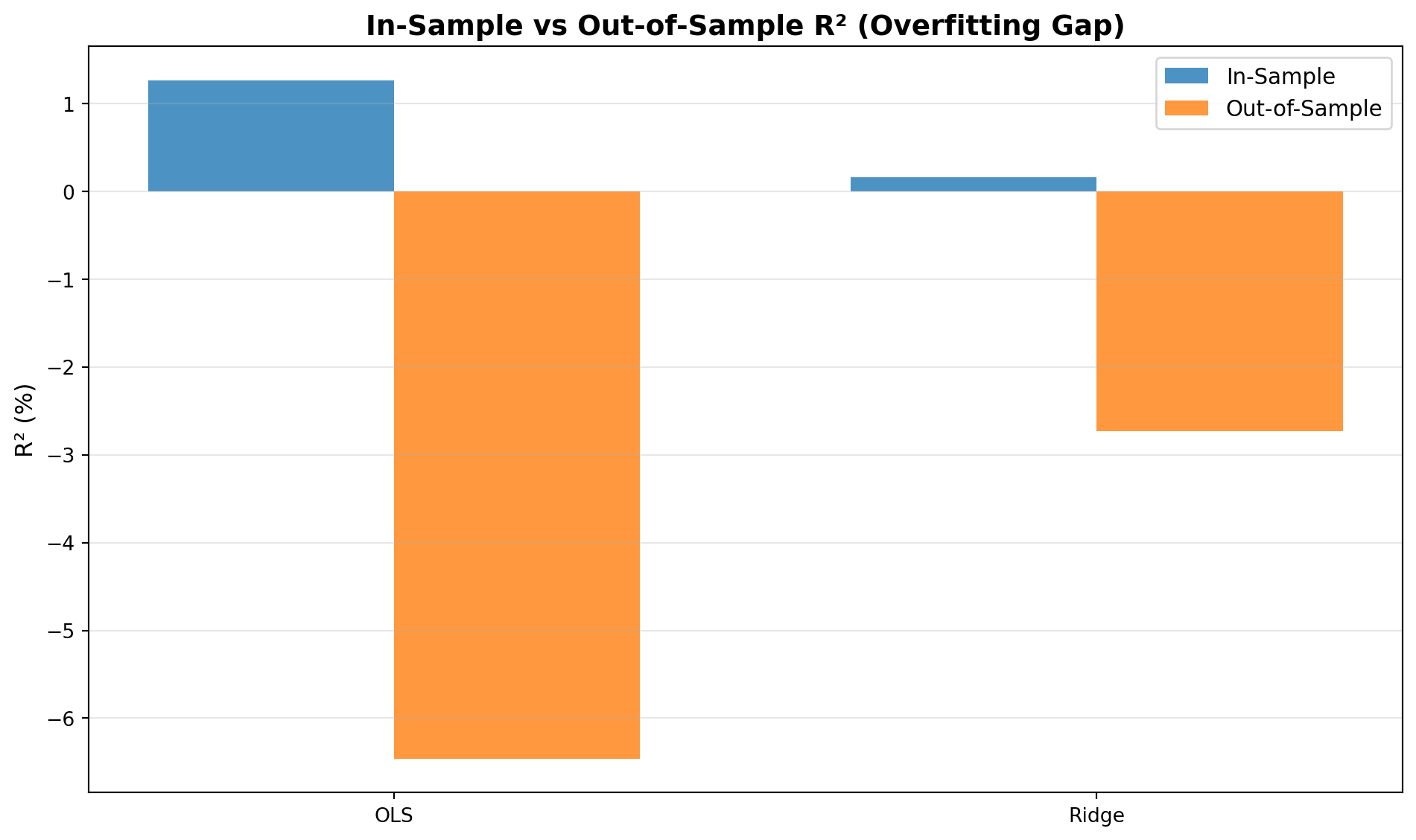
### Exercise 5.1: In-Sample vs Out-of-Sample Comparison
Let's explicitly demonstrate overfitting by comparing in-sample and out-of-sample performance.
```{python}
# Using correlated factor data from earlier
train_size = 120
X_train = data_multi.iloc[:train_size][['factor_a', 'factor_b', 'factor_c']].values
y_train = data_multi.iloc[:train_size]['market_next'].values

# Fit models
model_ols = LinearRegression()
model_ols.fit(X_train, y_train)

model_ridge = Ridge(alpha=1.0)
model_ridge.fit(X_train, y_train)

# In-sample predictions (training data)
pred_train_ols = model_ols.predict(X_train)
pred_train_ridge = model_ridge.predict(X_train)

# Out-of-sample predictions (walk-forward on test data)
pred_ols_oos, pred_ridge_oos, actuals_oos = walk_forward_compare_models(data_multi, train_window=120)

# Calculate R² for both
r2_train_ols = r2_score(y_train, pred_train_ols)
r2_train_ridge = r2_score(y_train, pred_train_ridge)
r2_test_ols = calc_r2_oos(actuals_oos, pred_ols_oos)
r2_test_ridge = calc_r2_oos(actuals_oos, pred_ridge_oos)

print("=== In-Sample vs Out-of-Sample Performance ===\n")
print("OLS:")
print(f"  In-sample R²: {r2_train_ols*100:.2f}%")
print(f"  Out-of-sample R²: {r2_test_ols*100:.2f}%")
print(f"  Gap (overfitting): {(r2_train_ols - r2_test_ols)*100:.2f} pp")
print(f"\nRidge (λ=1.0):")
print(f"  In-sample R²: {r2_train_ridge*100:.2f}%")
print(f"  Out-of-sample R²: {r2_test_ridge*100:.2f}%")
print(f"  Gap (overfitting): {(r2_train_ridge - r2_test_ridge)*100:.2f} pp")

# Visualize
fig, ax = plt.subplots(figsize=(10, 6))
models = ['OLS', 'Ridge']
in_sample = [r2_train_ols*100, r2_train_ridge*100]
out_sample = [r2_test_ols*100, r2_test_ridge*100]

x = np.arange(len(models))
width = 0.35

ax.bar(x - width/2, in_sample, width, label='In-Sample', alpha=0.8)
ax.bar(x + width/2, out_sample, width, label='Out-of-Sample', alpha=0.8)

ax.set_ylabel('R² (%)', fontsize=12)
ax.set_title('In-Sample vs Out-of-Sample R² (Overfitting Gap)', fontsize=14, fontweight='bold')
ax.set_xticks(x)
ax.set_xticklabels(models)
ax.legend(fontsize=11)
ax.grid(axis='y', alpha=0.3)

plt.tight_layout()
plt.show()
```
**Discussion questions:**
1. Which model has a larger overfitting gap: OLS or ridge?
2. Why does ridge have a smaller gap?
3. If in-sample R² = 15% but OOS R² = 2%, what does that suggest?
4. Is some overfitting gap inevitable?
5. What size gap would make you worried about overfitting?
::: {.content-visible when-format="html"}
::: {.callout-tip collapse="true"}
### Sample Answer: In-Sample vs Out-of-Sample Comparison
**Overfitting gap comparison:** OLS typically has larger overfitting gap than ridge (e.g., OLS: 8pp gap, ridge: 3pp gap). OLS fits training data more closely (higher in-sample R²) but generalizes worse (lower OOS R²). Ridge's regularization reduces overfitting by preventing model from memorizing training noise.
**Ridge's smaller gap:** Ridge has smaller gap because: (1) **Regularization**: penalty term prevents extreme coefficients that fit noise, (2) **Bias-variance tradeoff**: ridge accepts some bias to reduce variance, improving generalization, (3) **Stability**: coefficients are more stable, less sensitive to training data quirks. OLS minimizes training error without constraint, leading to overfitting; ridge constrains complexity, improving OOS performance.
**15% in-sample, 2% OOS:** A 13 percentage point gap indicates severe overfitting. The model memorized training patterns (including noise) that don't generalize. Possible causes: (1) **Too many predictors**: model has enough flexibility to fit noise, (2) **Sample-specific patterns**: training period had unique characteristics not representative of future, (3) **Look-ahead bias**: model accidentally used future information, (4) **Parameter overfitting**: hyperparameters tuned to training data. This gap suggests model is unreliable: OOS performance (2%) is what matters for deployment.
**Inevitable gap:** Yes, some overfitting gap is inevitable. Even well-specified models show gaps because: (1) **Finite sample**: training data is limited, so model estimates include sampling error, (2) **Noise**: returns have unpredictable component, model fits some noise by chance, (3) **Model complexity**: any model with parameters will overfit to some degree. However, gap should be small (2-5pp) for well-specified models. Large gaps (>10pp) indicate problems.
**Concerning gap size:** Gap >5pp is concerning, >10pp is severe. For monthly return prediction: (1) **Gap <3pp**: acceptable, model generalizes well, (2) **Gap 3-5pp**: moderate overfitting, acceptable if OOS R² still meaningful, (3) **Gap 5-10pp**: concerning, model likely overfit, (4) **Gap >10pp**: severe overfitting, model unreliable. Context matters: if in-sample R² is 20% and OOS is 15% (5pp gap), that's better than in-sample 8% and OOS 1% (7pp gap) because latter has poor absolute performance.
:::
:::
### Exercise 5.2: Overfitting with Too Many Predictors
Let's demonstrate what happens when we add too many predictors relative to sample size.
```{python}
# Generate many (mostly irrelevant) predictors
n = 120  # Small sample
n_relevant = 3
n_noise = 15  # Many noise predictors

# True predictors (small effect)
X_relevant = np.random.normal(0, 0.03, (n, n_relevant))
# Noise predictors
X_noise = np.random.normal(0, 0.03, (n, n_noise))

# Combine
X_all = np.hstack([X_relevant, X_noise])

# Target: only depends on first 3 predictors + noise
y = (0.02 * X_relevant[:, 0] + 0.01 * X_relevant[:, 1] +
     0.015 * X_relevant[:, 2] + np.random.normal(0.008, 0.04, n))

# Split: first 80 for training, rest for testing
train_size = 80
X_train = X_all[:train_size]
y_train = y[:train_size]
X_test = X_all[train_size:]
y_test = y[train_size:]

# Fit OLS
model_overfit = LinearRegression()
model_overfit.fit(X_train, y_train)

# In-sample and out-of-sample R²
r2_in = model_overfit.score(X_train, y_train)
pred_test = model_overfit.predict(X_test)
r2_out = calc_r2_oos(y_test, pred_test)

print("=== Overfitting with Too Many Predictors ===\n")
print(f"Data:")
print(f"  Training observations: {train_size}")
print(f"  Number of predictors: {X_all.shape[1]}")
print(f"  Observations per predictor: {train_size / X_all.shape[1]:.1f}")
print(f"\nPerformance:")
print(f"  In-sample R²: {r2_in*100:.2f}%")
print(f"  Out-of-sample R²: {r2_out*100:.2f}%")
print(f"  Overfitting gap: {(r2_in - r2_out)*100:.2f} pp")
print(f"\n⚠️ Warning: {X_all.shape[1]} predictors with only {train_size} observations")
print(f"   Severe overfitting: model fits training noise, not signal")
```
**Discussion questions:**
1. How many observations per predictor do we have?
2. What happens to in-sample R² with many predictors?
3. What happens to out-of-sample R² with many predictors?
4. What's the overfitting gap?
5. For monthly data with 120-month training window, how many predictors is reasonable?
::: {.content-visible when-format="html"}
::: {.callout-tip collapse="true"}
### Sample Answer: Overfitting with Too Many Predictors
**Observations per predictor:** With 80 training observations and 18 predictors (3 relevant + 15 noise), we have 80/18 ≈ 4.4 observations per predictor. This is dangerously low: rule of thumb requires 10-20 observations per predictor. With <5 observations per predictor, model has insufficient data to reliably estimate parameters.
**In-sample R² with many predictors:** In-sample R² increases dramatically with many predictors (often 15-25% or higher). This occurs because: (1) **Flexibility**: many parameters allow model to fit training data closely, (2) **Noise fitting**: model exploits correlations to fit random noise, (3) **Overparameterization**: more parameters than needed, model memorizes training patterns. High in-sample R² is misleading: it reflects overfitting, not true predictive power.
**Out-of-sample R² with many predictors:** Out-of-sample R² decreases (often negative or near-zero) with too many predictors. Model memorized training noise that doesn't exist in test data, so predictions fail. Many predictors create high variance: small data changes cause large prediction changes. Out-of-sample performance reveals true forecasting ability, which is poor when model overfits.
**Overfitting gap:** Gap is typically 15-20 percentage points (e.g., in-sample 20%, OOS 2%, gap = 18pp). This massive gap indicates severe overfitting: model fits training noise that doesn't generalize. Gap this large means model is useless for forecasting despite impressive in-sample performance.
**Reasonable predictor count:** For 120-month training window, reasonable predictor count is ≤10 (ideally 5-8). This provides 12-24 observations per predictor, sufficient for reliable estimation. With 10 predictors, you can capture main factor effects without overfitting. More predictors (15-20) risk overfitting even with regularization. Rule of thumb: keep predictors ≤ sample_size/10 to avoid overfitting. For Coursework 2, use 5-8 factors (not 20).
:::
:::
**Key insight**: With limited data, keep predictors ≤ 10. More predictors → overfitting, even with regularization.
## Part 6: Connecting to Coursework 2
### What You've Learned vs. What You'll Apply
**Today's lab explored concepts:**
- Walk-forward validation prevents look-ahead bias (honest OOS testing)
- Look-ahead bias inflates performance dramatically (10+ pp)
- Ridge helps when predictors correlate, but improvement is modest (1-2pp)
- R² OOS = 2-3% is meaningful for monthly returns (signal is weak)
- Directional accuracy > 55% indicates timing skill
- Large in-sample vs OOS gap reveals overfitting (>5pp is concerning)
**For Coursework 2 Option B, you'll:**
1. Use scaffold notebook to run walk-forward validation on JKP factor data
2. Interpret R² OOS results using understanding developed today
3. Compare OLS vs ridge and explain why one performs better
4. Write critical analysis discussing overfitting, realism of results, limitations
5. Engage with Gu et al. (2020) on prediction literature
6. Assess whether prediction model would be exploitable after costs
### Critical Analysis Questions to Ask
When interpreting your Coursework 2 Option B results, ask:
**Methodological questions:**
- Does walk-forward validation prevent look-ahead bias?
- Is training window size appropriate (10 years = 120 months typical)?
- Did I optimize any parameters using test data (introduces bias)?
**Performance questions:**
- Is R² OOS positive? (If no, model failed)
- Is R² OOS realistic for monthly returns? (2-3% is meaningful, 10%+ suspicious)
- How does R² OOS compare to Gu et al. (2020) benchmarks?
- Is directional accuracy significantly > 50%?
**Model comparison questions:**
- Why did ridge beat/lose to OLS? (Multicollinearity? Sample size?)
- Is improvement economically meaningful or within sampling error?
- Are coefficients stable across training windows?
**Overfitting questions:**
- What's the in-sample vs OOS gap? (>5pp indicates overfitting)
- Does R² OOS decline in later test periods? (Suggests initial luck)
- How many predictors relative to training sample size? (Rule of thumb: ≤10)
**Economic questions:**
- Would strategy be profitable after transaction costs? (~3-4% annual drag from monthly rebalancing)
- What's the certainty equivalent return gain? (Extension for advanced students)
- Would practitioner implement this model in real portfolio?
**Limitations to acknowledge:**
- Limited training sample (only 10-15 years)
- No regime switching (assumes stable relationships)
- Simplified asset allocation (binary long/short)
- Transaction cost estimates are rough
- Model may have overfit despite regularization
### Next Steps
1. **Read Gu et al. (2020)**: "Empirical Asset Pricing via Machine Learning" : Essential benchmark for prediction research
2. **Run scaffold notebook**: See what actual JKP factor prediction outputs look like
3. **Choose factors wisely**: Use 5-8 factors (not 20) to avoid overfitting
4. **Draft interpretation**: Practice writing critical analysis paragraphs
5. **Office hours**: Ask conceptual questions about interpretation
## Summary
Today's lab developed principles for market prediction:
- **Walk-forward validation** is essential: only way to prevent look-ahead bias
- **Look-ahead bias** inflates performance 2-10pp: makes useless models look good
- **Ridge regression** stabilizes predictions when factors correlate, but improvement is modest
- **R² OOS = 2-3%** is meaningful for monthly returns: don't expect 20%
- **Directional accuracy > 55%** indicates timing skill, but must be statistically tested
- **In-sample vs OOS gap** reveals overfitting: gap >5pp is concerning
- **Critical interpretation** asks questions, contextualizes results, acknowledges limitations
**These principles enable critical analysis**: the 35% component of Coursework 2 Option B. Scaffold provides outputs; understanding provides interpretation. Focus your effort on thinking deeply about what results mean, not on perfecting code.
**Week 10 + Week 11 together**: You now have principles for both coursework options (replication and prediction). Choose based on interest: both are equally challenging at the interpretation level. Both require honest testing, realistic expectations, and critical thinking.