---
title: "Robo-Advisers and Portfolio Optimisation"
author: "Professor Barry Quinn"
date: today
format:
html:
code-fold: true
code-summary: "Show Python code"
code-tools:
source: true
toggle: true
caption: none
execute:
warning: false
message: false
echo: true
eval: true
fig-width: 10
fig-height: 6
fig-format: png
jupyter: fin510
bibliography:
- ../resources/reading.bib
- ../resources/reading_supp.bib
---
**Theme**: Modern Investment & Financial Inclusion
::: {.callout-note}
#### View Slides
Open the lecture deck: [Robo-Advisers & Portfolio Optimisation](../slides/week05_robo.qmd)
:::
```{python}
#| label: setup-data-root
#| include: false
import sys
from pathlib import Path
import yaml
sys.path.insert(0, str(Path("scripts").resolve()))
from bloomberg_loader import load_bloomberg
try:
with open(Path("config/data_root.yml")) as f:
cfg = yaml.safe_load(f)
data_root = Path(cfg.get("data_root", "data")).expanduser().resolve()
except Exception:
data_root = Path("data")
```
# Introduction: The Algorithmic Revolution in Investment Management
The democratisation of investment management through robo-advisers has emerged as one of the most visible applications of FinTech innovation. Its long-term significance will depend on sustained adoption, regulatory frameworks, and the ability of these models to deliver consistent value. By combining the data acquisition capabilities we developed in Week 2 with sophisticated algorithmic portfolio management, robo-advisers have made professional-quality investment advice accessible to investors who were previously underserved by traditional wealth management.
Recent research by @reher2024robo provides compelling evidence that robo-advisers expand access to wealth management for middle-class investors by lowering account minimums, creating measurable welfare gains for previously underserved segments. Their quasi-experimental analysis demonstrates that when robo-advisers reduce minimum investment requirements, participation rates increase significantly among investors with moderate wealth levels.
These welfare effects are modest in size, concentrated among middle-class investors with sufficient investable wealth, and sensitive to both institutional design and behavioural responses.
This expansion of access reflects the broader theme we established in Week 1's analysis of FinTech innovation. Just as @berg2020credit showed how FinTech lenders use superior data processing to serve previously excluded borrowers, robo-advisers use algorithmic portfolio management to serve investors that traditional wealth managers found unprofitable.
But the story of robo-advisers is more than just democratisation. The underlying algorithms represent a practical application of the computational complexity insights we discussed in our Data Science Primer. As @gu2020ml demonstrate in their foundational work on "Empirical Asset Pricing via Machine Learning," sophisticated algorithms can capture patterns in financial data that simpler approaches miss, potentially improving investment outcomes for all types of investors.
### From Characteristics to Embeddings: Learning Asset Relationships
Traditional portfolio construction relies on observable firm characteristics: size, book-to-market ratios, momentum, profitability. But what if we could learn asset relationships directly from how professional investors actually construct portfolios? Recent work by @gabaix2025assetembeddings shows that portfolio holdings themselves encode rich information about which assets belong together.
The intuition mirrors how natural language processing learns word meanings. Words appearing in similar contexts (like "bank" and "river" both appearing near "water") have related meanings. Similarly, assets appearing in similar portfolios (Apple and Microsoft both held by growth-focused technology funds) share investment characteristics. By analyzing thousands of institutional portfolios, embedding models learn compressed representations: high-dimensional vectors capturing each asset's "investment profile": without requiring hand-crafted features.
This approach offers three advantages for algorithmic investment management. First, embeddings automatically incorporate information that might be difficult to encode as explicit characteristics: industry relationships, supply chain connections, management quality signals reflected in professional investors' revealed preferences. Second, embeddings update continuously as new holdings data arrives, adapting to evolving market structure without manual feature engineering. Third, embeddings enable recommendation-system approaches: suggesting portfolio additions based on similarity to existing holdings, the same technology powering Netflix recommendations or Amazon product suggestions.
The welfare implications connect to @reher2024robo's findings about robo-advisors expanding access. If embeddings enable better portfolio construction at lower marginal cost: learning from institutional behavior without requiring expensive fundamental research: they potentially extend sophisticated investment strategies to middle-class investors previously excluded from personalized portfolio management. Whether this theoretical potential translates to practice remains an empirical question, but the approach illustrates how machine learning techniques originally developed for consumer applications (recommendations, search) are being adapted to financial contexts with meaningful distributional consequences.
#
## Learning objectives
By the end of this week, you should be able to:
- Contrast traditional advisory and robo‑advisory models, including economic drivers of access and cost.
- Implement and interpret simple analyses of cost structures and portfolio choices.
- Explain welfare and inclusion implications using recent empirical evidence (@reher2024robo) with appropriate caveats.
- Identify key risks and governance considerations (suitability, disclosure, bias) for algorithmic advice.
# Part I: The Economics of Robo-Advisory Services
## Understanding the Traditional Wealth Management Model
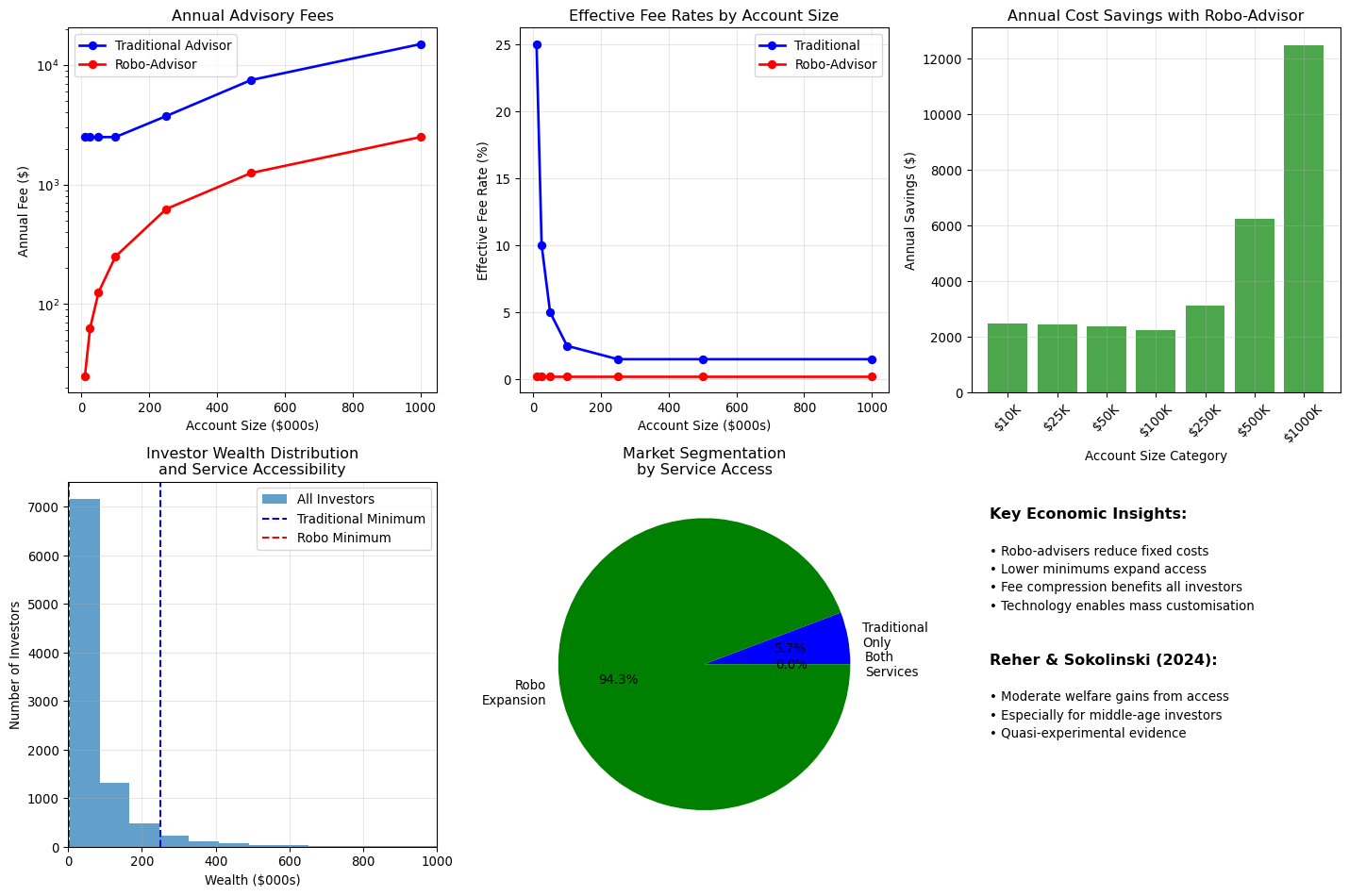
Traditional wealth management operates on a high-touch, relationship-based model that requires significant human resources. Financial advisers typically charge fees of 1-1.5% of assets under management and often require minimum account sizes of $250,000 or more to ensure profitability.
This model creates natural barriers to access. As @hilpisch2019 observes in his analysis of financial technology barriers, traditional advisory services require "investments of $25-36 million just for derivatives analytics libraries, along with teams of experts who understand both finance and technology." Whilst this refers to sophisticated trading systems, the principle applies broadly: high-touch financial services require substantial fixed costs that must be amortised across large account balances.
The traditional model also faces scalability constraints. Human advisers can only manage a limited number of client relationships effectively, creating capacity constraints that push firms towardss serving higher-net-worth clients who generate more revenue per relationship.
# *Note:* The following analysis uses stylised assumptions for teaching purposes. Actual advisory fee structures and minimums vary significantly across firms and jurisdictions.
```{python}
# Analyzing the economics of traditional vs. robo-advisory services
import pandas as pd
import numpy as np
import matplotlib.pyplot as plt

def analyse_advisory_economics():
    """
    Compare the cost structures of traditional vs. robo-advisory services
    """
    print("Economics of Traditional vs. Robo-Advisory Services")
    print("=" * 55)

    # Define cost structures
    account_sizes = np.array([10000, 25000, 50000, 100000, 250000, 500000, 1000000])

    # Traditional advisor costs
    traditional_fee_rate = 0.015  # 1.5% AUM
    traditional_minimum_fee = 2500  # Minimum annual fee
    traditional_fees = np.maximum(account_sizes * traditional_fee_rate, traditional_minimum_fee)

    # Robo-advisor costs
    robo_fee_rate = 0.0025  # 0.25% AUM
    robo_minimum_fee = 0  # No minimum
    robo_fees = account_sizes * robo_fee_rate

    # Calculate effective fee rates
    traditional_effective_rates = traditional_fees / account_sizes
    robo_effective_rates = robo_fees / account_sizes

    print("Cost Analysis by Account Size:")
    print("=" * 60)
    print(f"{'Account Size':<15} {'Traditional':<12} {'Robo':<12} {'Savings':<12} {'Rate Diff':<12}")
    print("-" * 60)

    for i, size in enumerate(account_sizes):
        traditional_cost = traditional_fees[i]
        robo_cost = robo_fees[i]
        savings = traditional_cost - robo_cost
        rate_diff = traditional_effective_rates[i] - robo_effective_rates[i]

        # Width before grouping option; left-align for the size column
        print(f"${size:<14,} ${traditional_cost:>8,.0f} ${robo_cost:>8,.0f} ${savings:>8,.0f} {rate_diff*100:>8.2f}%")

    # Identify break-even point for traditional advisers
    break_even = traditional_minimum_fee / traditional_fee_rate
    print(f"\nTraditional advisor break-even account size: ${break_even:,.0f}")

    # Visualization
    plt.figure(figsize=(15, 10))

    # Annual fees comparison
    plt.subplot(2, 3, 1)
    plt.plot(account_sizes/1000, traditional_fees, 'b-o', label='Traditional Advisor', linewidth=2)
    plt.plot(account_sizes/1000, robo_fees, 'r-o', label='Robo-Advisor', linewidth=2)
    plt.xlabel('Account Size ($000s)')
    plt.ylabel('Annual Fee ($)')
    plt.title('Annual Advisory Fees')
    plt.legend()
    plt.grid(True, alpha=0.3)
    plt.yscale('log')

    # Effective fee rates
    plt.subplot(2, 3, 2)
    plt.plot(account_sizes/1000, traditional_effective_rates*100, 'b-o', label='Traditional', linewidth=2)
    plt.plot(account_sizes/1000, robo_effective_rates*100, 'r-o', label='Robo-Advisor', linewidth=2)
    plt.xlabel('Account Size ($000s)')
    plt.ylabel('Effective Fee Rate (%)')
    plt.title('Effective Fee Rates by Account Size')
    plt.legend()
    plt.grid(True, alpha=0.3)

    # Cost savings
    plt.subplot(2, 3, 3)
    savings = traditional_fees - robo_fees
    plt.bar(range(len(account_sizes)), savings, alpha=0.7, color='green')
    plt.xlabel('Account Size Category')
    plt.ylabel('Annual Savings ($)')
    plt.title('Annual Cost Savings with Robo-Advisor')
    plt.xticks(range(len(account_sizes)), [f'${s/1000:.0f}K' for s in account_sizes], rotation=45)
    plt.grid(True, alpha=0.3)

    # Access analysis
    plt.subplot(2, 3, 4)
    # Simulate investor distribution (log-normal)
    np.random.seed(42)
    investor_wealth = np.random.lognormal(mean=10.5, sigma=1.2, size=10000)  # Wealth distribution
    investor_wealth = investor_wealth[investor_wealth >= 5000]  # Minimum for any service

    # Traditional access (minimum $250K effectively due to fees)
    traditional_accessible = investor_wealth[investor_wealth >= 250000]
    robo_accessible = investor_wealth[investor_wealth >= 1000]  # Much lower minimum

    print(f"\nAccess Analysis (Simulated Investor Population):")
    print(f"  Total investors (>$5K): {len(investor_wealth):,}")
    print(f"  Traditional advisor access: {len(traditional_accessible):,} ({len(traditional_accessible)/len(investor_wealth)*100:.1f}%)")
    print(f"  Robo-advisor access: {len(robo_accessible):,} ({len(robo_accessible)/len(investor_wealth)*100:.1f}%)")
    print(f"  Additional access from robo: {len(robo_accessible) - len(traditional_accessible):,} investors")

    plt.hist(investor_wealth/1000, bins=50, alpha=0.7, label='All Investors')
    plt.axvline(250, color='blue', linestyle='--', label='Traditional Minimum')
    plt.axvline(1, color='red', linestyle='--', label='Robo Minimum')
    plt.xlabel('Wealth ($000s)')
    plt.ylabel('Number of Investors')
    plt.title('Investor Wealth Distribution\nand Service Accessibility')
    plt.legend()
    plt.xlim(0, 1000)
    plt.grid(True, alpha=0.3)

    # Market opportunity
    plt.subplot(2, 3, 5)
    categories = ['Traditional\nOnly', 'Robo\nExpansion', 'Both\nServices']
    sizes = [
        len(traditional_accessible),
        len(robo_accessible) - len(traditional_accessible),
        len(investor_wealth) - len(robo_accessible)
    ]
    colors = ['blue', 'green', 'grey']

    plt.pie(sizes, labels=categories, colors=colors, autopct='%1.1f%%')
    plt.title('Market Segmentation\nby Service Access')

    # Key insights
    plt.subplot(2, 3, 6)
    plt.text(0.05, 0.9, 'Key Economic Insights:', fontweight='bold', fontsize=12)
    plt.text(0.05, 0.8, '• Robo-advisers reduce fixed costs', fontsize=10)
    plt.text(0.05, 0.75, '• Lower minimums expand access', fontsize=10)
    plt.text(0.05, 0.7, '• Fee compression benefits all investors', fontsize=10)
    plt.text(0.05, 0.65, '• Technology enables mass customisation', fontsize=10)

    plt.text(0.05, 0.5, 'Reher & Sokolinski (2024):', fontweight='bold', fontsize=12)
    plt.text(0.05, 0.4, '• Moderate welfare gains from access', fontsize=10)
    plt.text(0.05, 0.35, '• Especially for middle-age investors', fontsize=10)
    plt.text(0.05, 0.3, '• Quasi-experimental evidence', fontsize=10)

    plt.xlim(0, 1)
    plt.ylim(0, 1)
    plt.axis('off')

    plt.tight_layout()
    plt.show()

    return {
        'account_sizes': account_sizes,
        'traditional_fees': traditional_fees,
        'robo_fees': robo_fees,
        'access_expansion': len(robo_accessible) - len(traditional_accessible)
    }

# Run the analysis
advisory_economics = analyse_advisory_economics()
```
This economic analysis demonstrates why robo-advisers represent more than just technological innovation: they fundamentally change the economics of investment advice delivery, enabling what @vives2019banking categorises as "product innovation" that serves previously underserved markets.
## The Technology Behind Robo-Advisory Services
Robo-advisers succeed by automating the core functions of traditional investment management: portfolio construction, rebalancing, tax-loss harvesting, and performance monitoring. This automation is possible because many investment management decisions can be systematised using well-established financial theory and computational methods.
The technological foundation draws heavily on Modern Portfolio Theory, as implemented in @hilpisch2019's Chapter 13 on portfolio analytics. However, modern robo-advisers extend these classical approaches with machine learning techniques for improved risk assessment, behavioural analysis for better client outcomes, and automated execution for efficient implementation.
### Portfolio optimisation Algorithms
The core of most robo-advisory services is an automated portfolio optimisation engine that implements variations of Modern Portfolio Theory. These systems take client risk preferences, investment objectives, and constraints as inputs and produce optimal portfolio allocations as outputs.
::: {.callout-warning}
## Connection to Data & Measurement ([Week 2, §2.3](02_data_measurement.qmd#selection-bias))
**Survivorship bias in equity data**: When we calculate historical returns from equity indices (S&P 500, FTSE 100), we only observe survivors. Failed companies disappear from the index, creating upward bias in estimated returns.
**Example**: S&P 500 returns 1990-2020 exclude companies that went bankrupt, were acquired, or delisted. If we base portfolio optimization on these survivorship-biased returns, we'll overestimate expected performance.
**Mitigation**:
- Use point-in-time indices that reflect actual investable universe at each date
- Bloomberg Terminal provides "backfilled" vs "point-in-time" data options
- Adjust expected returns downward to account for survivor bias (typically -1% to -2% per year)
Recall our Week 2 lab where we quantified survivorship bias in UK banking crisis data: the same principle applies to equity portfolios.
:::
::: {.callout-tip}
## Connection to Volatility Modeling ([Week 3, §3.2](03_volatility_modelling.qmd#garch-models))
**Covariance matrices are not constant**: Recall from Chapter 03 that volatility exhibits clustering (GARCH effects) and time-variation. The same applies to covariances.
**Problem**: We estimate covariance on historical data (e.g., 2015-2020), assuming it's stable. But correlations are not constant: during crisis periods, correlations spike toward 1 as all assets fall together; during calm periods, correlations are lower and diversification works better; and regime shifts (such as the 2020 pandemic) can alter correlations permanently.
**Implication**: Optimal weights based on calm-period covariances will fail during crises when correlations surge. This is why "diversified" portfolios crash together during market stress.
**Solutions**:
- Dynamic conditional correlation (DCC-GARCH) from Ch 03: model time-varying correlations
- Stress-test portfolios using crisis-period covariances
- Use rolling windows to adapt to changing correlations
:::
# **Caution.** This behavioural simulation is highly stylised. Real investor behaviour is shaped by cultural, institutional, and macroeconomic contexts, and robo-advisor effectiveness in mitigating biases depends on actual client engagement and platform design.
```{python}
# Implementing robo-advisor portfolio optimisation
import pandas as pd
import numpy as np
import os
import matplotlib.pyplot as plt
from scipy.optimize import minimize

class RoboAdvisorEngine:
    """
    Basic robo-advisor portfolio optimisation engine
    Following Hilpisch Chapter 13 portfolio analytics approach
    """

    def __init__(self, symbols, risk_free_rate=0.02):
        self.symbols = symbols
        self.risk_free_rate = risk_free_rate
        self.returns_data = None
        self.expected_returns = None
        self.cov_matrix = None

    def fetch_market_data(self):
        """
        Load market data from Bloomberg database
        """
        print(f"Loading data for {len(self.symbols)} assets from Bloomberg database...")

        try:
            # Load from Bloomberg database
            bbg = load_bloomberg()

            price_data = {}
            for symbol in self.symbols:
                ticker_data = bbg[bbg['ticker'] == symbol].copy()
                if ticker_data.empty:
                    raise ValueError(f"Ticker {symbol} not found in database")
                ticker_data['date'] = pd.to_datetime(ticker_data['date'])
                ticker_data = ticker_data.set_index('date').sort_index()
                price_data[symbol] = ticker_data['PX_LAST']

            price_data = pd.DataFrame(price_data)

            if price_data.empty:
                raise ValueError("No price data available")

            # Calculate returns
            self.returns_data = price_data.pct_change().dropna()

            # Estimate expected returns (simple historical mean)
            self.expected_returns = self.returns_data.mean() * 252  # Annualized

            # Estimate covariance matrix
            self.cov_matrix = self.returns_data.cov() * 252  # Annualized

            # Note: These are ESTIMATES with substantial uncertainty
            # Standard errors for expected returns are typically 5-15% annualized
            # This uncertainty propagates to optimal weights (see sensitivity analysis below)

            print("Successfully prepared data:")
            print(f"   Trading days: {len(self.returns_data)}")
            print(f"   Assets: {len(self.symbols)}")
            print(f"   Expected returns range: {self.expected_returns.min()*100:.1f}% to {self.expected_returns.max()*100:.1f}%")

            return True

        except Exception as e:
            print(f"Error fetching market data: {e}")
            return False

    def optimize_portfolio(self, target_return=None, risk_aversion=None):
        """
        Optimize portfolio using Modern Portfolio Theory
        """
        if self.expected_returns is None or self.cov_matrix is None:
            print("No market data available. Run fetch_market_data() first.")
            return None

        n_assets = len(self.symbols)

        # Objective function for portfolio optimisation
        def portfolio_volatility(weights):
            """Calculate portfolio volatility"""
            return np.sqrt(np.dot(weights.T, np.dot(self.cov_matrix, weights)))

        def portfolio_return(weights):
            """Calculate expected portfolio return"""
            return np.dot(weights, self.expected_returns)

        def sharpe_ratio(weights):
            """Calculate negative Sharpe ratio (for minimization)"""
            port_return = portfolio_return(weights)
            port_vol = portfolio_volatility(weights)
            if port_vol == 0:
                return -np.inf
            return -(port_return - self.risk_free_rate) / port_vol

        # Constraints
        constraints = [
            {'type': 'eq', 'fun': lambda x: np.sum(x) - 1}  # Weights sum to 1
        ]

        if target_return is not None:
            constraints.append({
                'type': 'eq',
                'fun': lambda x: portfolio_return(x) - target_return
            })

        # Bounds (no short selling, max 40% in any single asset)
        bounds = [(0, 0.4) for _ in range(n_assets)]

        # Initial guess (equal weights)
        initial_weights = np.array([1/n_assets] * n_assets)

        # Optimize
        if risk_aversion is not None:
            # Risk-averse optimisation (minimise variance for given return preference)
            def objective(weights):
                return portfolio_volatility(weights)**2 + risk_aversion * (-portfolio_return(weights))
        else:
            # Maximize Sharpe ratio
            objective = sharpe_ratio

        try:
            result = minimize(
                objective,
                initial_weights,
                method='SLSQP',
                bounds=bounds,
                constraints=constraints,
                options={'maxiter': 1000}
            )

            if result.success:
                optimal_weights = result.x
                opt_return = portfolio_return(optimal_weights)
                opt_vol = portfolio_volatility(optimal_weights)
                opt_sharpe = (opt_return - self.risk_free_rate) / opt_vol

                print("\nPortfolio optimisation successful:")
                print(f"   Expected return: {opt_return*100:.2f}%")
                print(f"   Volatility: {opt_vol*100:.2f}%")
                print(f"   Sharpe ratio: {opt_sharpe:.3f}")

                # Show allocation
                print(f"\n   Optimal Allocation:")
                for symbol, weight in zip(self.symbols, optimal_weights):
                    if weight > 0.01:  # Only show significant allocations
                        print(f"     {symbol}: {weight*100:.1f}%")

                return {
                    'weights': optimal_weights,
                    'expected_return': opt_return,
                    'volatility': opt_vol,
                    'sharpe_ratio': opt_sharpe
                }
            else:
                print(f"Optimisation failed: {result.message}")
                return None

        except Exception as e:
            print(f"Optimisation error: {e}")
            return None

    def generate_efficient_frontier(self, n_portfolios=50):
        """
        Generate efficient frontier for visualisation
        """
        if self.expected_returns is None:
            print("No market data available")
            return None

        print(f"Generating efficient frontier with {n_portfolios} portfolios...")

        # Range of target returns
        min_return = self.expected_returns.min()
        max_return = self.expected_returns.max()
        target_returns = np.linspace(min_return, max_return, n_portfolios)

        efficient_portfolios = []

        for target in target_returns:
            # Optimize for this target return
            result = self.optimize_portfolio(target_return=target)
            if result:
                efficient_portfolios.append({
                    'target_return': target,
                    'volatility': result['volatility'],
                    'sharpe_ratio': result['sharpe_ratio'],
                    'weights': result['weights']
                })

        if efficient_portfolios:
            print(f"Generated {len(efficient_portfolios)} efficient portfolios")
            return pd.DataFrame(efficient_portfolios)
        else:
            print("Failed to generate efficient frontier")
            return None

# Demonstrate robo-advisor optimisation
def demonstrate_robo_optimization():
    """
    Demonstrate robo-advisor portfolio optimisation capabilities
    """
    print("Robo-Advisor Portfolio optimisation Demonstration")
    print("=" * 55)

    # Define a diversified ETF portfolio (typical robo-advisor approach)
    etf_portfolio = {
        'VTI': 'Total Stock Market',
        'VTIAX': 'International Stocks',
        'BND': 'Total Bond Market',
        'VNQ': 'Real Estate (REITs)',
        'VDE': 'Energy Sector',
        'VGT': 'Technology Sector'
    }

    symbols = list(etf_portfolio.keys())

    # Create robo-advisor engine
    robo = RoboAdvisorEngine(symbols)

    # Fetch data and optimise
    if robo.fetch_market_data():

        # Optimize for maximum Sharpe ratio
        optimal_portfolio = robo.optimize_portfolio()

        if optimal_portfolio:
            # Generate efficient frontier
            efficient_frontier = robo.generate_efficient_frontier(n_portfolios=30)

            if efficient_frontier is not None:
                # Visualization
                plt.figure(figsize=(12, 8))

                # Efficient frontier
                plt.subplot(2, 2, 1)
                plt.plot(efficient_frontier['volatility']*100,
                        efficient_frontier['target_return']*100,
                        'b-', linewidth=2, label='Efficient Frontier')

                # Highlight optimal portfolio
                plt.plot(optimal_portfolio['volatility']*100,
                        optimal_portfolio['expected_return']*100,
                        'ro', markersize=10, label='Optimal (Max Sharpe)')

                plt.xlabel('Volatility (%)')
                plt.ylabel('Expected Return (%)')
                plt.title('Efficient Frontier')
                plt.legend()
                plt.grid(True, alpha=0.3)

                # Portfolio allocation
                plt.subplot(2, 2, 2)
                weights = optimal_portfolio['weights']
                significant_weights = [(symbols[i], w) for i, w in enumerate(weights) if w > 0.01]

                if significant_weights:
                    labels, values = zip(*significant_weights)
                    plt.pie(values, labels=labels, autopct='%1.1f%%')
                    plt.title('Optimal Portfolio Allocation')

                # Sharpe ratio across frontier
                plt.subplot(2, 2, 3)
                plt.plot(efficient_frontier['volatility']*100,
                        efficient_frontier['sharpe_ratio'],
                        'g-', linewidth=2)
                plt.axhline(optimal_portfolio['sharpe_ratio'], color='red', linestyle='--',
                           label=f'Max Sharpe: {optimal_portfolio["sharpe_ratio"]:.3f}')
                plt.xlabel('Volatility (%)')
                plt.ylabel('Sharpe Ratio')
                plt.title('Sharpe Ratio vs Risk')
                plt.legend()
                plt.grid(True, alpha=0.3)

                # Expected returns by asset
                plt.subplot(2, 2, 4)
                asset_returns = robo.expected_returns * 100
                colors = ['green' if r > 0 else 'red' for r in asset_returns]
                bars = plt.bar(range(len(symbols)), asset_returns, color=colors, alpha=0.7)
                plt.xlabel('Assets')
                plt.ylabel('Expected Return (%)')
                plt.title('Expected Returns by Asset')
                plt.xticks(range(len(symbols)), symbols, rotation=45)
                plt.grid(True, alpha=0.3)

                plt.tight_layout()
                plt.show()

                print("\nRobo-adviser insights:")
                print(f"  - Automated optimisation enables low-cost advice")
                print(f"  - Diversification reduces risk without sacrificing return")
                print(f"  - Systematic approach removes emotional biases")
                print(f"  - Scalable technology serves mass market")

# Run the demonstration
demonstrate_robo_optimization()
```
This analysis demonstrates the core technological capability that enables robo-advisers to serve mass markets cost-effectively. By automating portfolio optimisation, these services can provide sophisticated investment advice at a fraction of traditional costs.
### The Problem with Naive Optimization: Estimation Error
The portfolio optimization we just implemented has a critical flaw: **it treats estimated parameters (expected returns, covariances) as if they were true values**. This ignores estimation error and leads to unstable, poorly performing portfolios.
::: {.callout-warning}
## Connection to Statistical Foundations ([Week 1, §0.2](01_foundations.qmd#bias-variance-tradeoff))
Recall Gelman's principle: **"All parameters are estimated with uncertainty."** When we compute expected returns from historical data, we get estimates μ̂ with standard errors. A stock with 10% historical return might truly have 8% or 12% expected return.
**The problem**: Portfolio optimization is **extremely sensitive** to small changes in inputs. A 1% change in expected return can shift optimal weights by 20-30 percentage points. Estimation error in inputs → massive uncertainty in outputs.
**Why this matters**: In-sample optimization produces weights that look optimal for historical data, but out-of-sample reality reveals that performance collapses because the estimates were wrong, reflecting overfitting where the optimizer exploits noise in the data rather than real patterns.
This is the **bias-variance tradeoff**. Unconstrained optimization (low bias) overfits to noise (high variance). We need regularization.
:::
```{python}
# Demonstrate estimation error sensitivity
def sensitivity_analysis(engine, perturbation=0.01):
    """Show how small changes in expected returns affect optimal weights"""
    print(f"\n=== Sensitivity Analysis: Impact of Estimation Error ===\n")

    # Baseline optimization
    baseline = engine.optimize_portfolio()
    if baseline is None:
        return

    baseline_weights = baseline['weights']
    original_returns = engine.expected_returns.copy()

    # Perturb returns by ±1% (within estimation error)
    engine.expected_returns = original_returns + perturbation
    perturbed_up = engine.optimize_portfolio()

    engine.expected_returns = original_returns - perturbation
    perturbed_down = engine.optimize_portfolio()

    engine.expected_returns = original_returns  # Restore

    if perturbed_up and perturbed_down:
        weight_change_up = perturbed_up['weights'] - baseline_weights
        weight_change_down = perturbed_down['weights'] - baseline_weights

        print(f"Perturbation: ±{perturbation*100:.1f}% to all expected returns")
        print(f"\nMaximum weight change:")
        print(f"  +{perturbation*100:.0f}% perturbation: {np.abs(weight_change_up).max()*100:.1f} pp")
        print(f"  -{perturbation*100:.0f}% perturbation: {np.abs(weight_change_down).max()*100:.1f} pp")
        print(f"\nNote: a {perturbation*100:.0f}% error in expected returns (well within estimation error)")
        print(f"  causes {np.abs(weight_change_up).max()*100:.0f}pp weight changes: portfolios are VERY unstable!")

# Run demonstration
symbols = ['SPY', 'TLT', 'GLD', 'VNQ']
engine = RoboAdvisorEngine(symbols)
if engine.fetch_market_data():
    sensitivity_analysis(engine, perturbation=0.01)
```
::: {.callout-tip}
## Connection to Statistical Foundations (Week 1, §0.2 & Ch 02, §2.2)
This demonstrates **parameter uncertainty propagation**: Small uncertainty in inputs → large uncertainty in outputs.
**Why optimization is so sensitive**:
- High dimensionality (with 50 assets, covariance matrix has 1,275 parameters)
- Optimizer exploits tiny differences in expected returns
- No shrinkage: treats noise as signal
**Data quality matters** (Ch 02): Historical returns suffer from survivorship bias (failed stocks excluded from indices), measurement error (returns calculated from noisy prices), and non-stationarity (past returns do not equal future returns).
The solution: **Regularisation** (constraints, shrinkage) or **Bayesian methods** (acknowledge uncertainty explicitly).
:::
### Solution 1: Bootstrap Confidence Intervals for Weights
To quantify uncertainty, we can bootstrap the return data and see how optimal weights vary across resampled datasets.
```{python}
def bootstrap_portfolio_weights(engine, n_bootstrap=200):
    """
    Bootstrap confidence intervals for optimal portfolio weights
    """
    print(f"\n=== Bootstrap Analysis ({n_bootstrap} iterations) ===\n")

    if engine.returns_data is None:
        print("No data available")
        return

    returns = engine.returns_data
    n_obs, n_assets = returns.shape

    bootstrap_weights = []

    # Bootstrap resampling
    np.random.seed(42)
    for i in range(n_bootstrap):
        # Resample with replacement
        indices = np.random.choice(n_obs, size=n_obs, replace=True)
        resampled_returns = returns.iloc[indices]

        # Re-estimate parameters
        engine.expected_returns = resampled_returns.mean() * 252
        engine.cov_matrix = resampled_returns.cov() * 252

        # Re-optimize
        result = engine.optimize_portfolio()
        if result:
            bootstrap_weights.append(result['weights'])

    if not bootstrap_weights:
        print("Bootstrap failed")
        return

    bootstrap_weights = np.array(bootstrap_weights)

    # Calculate statistics
    mean_weights = bootstrap_weights.mean(axis=0)
    std_weights = bootstrap_weights.std(axis=0)
    ci_lower = np.percentile(bootstrap_weights, 2.5, axis=0)
    ci_upper = np.percentile(bootstrap_weights, 97.5, axis=0)

    print(f"Bootstrap Results ({n_bootstrap} iterations):\n")
    print(f"{'Asset':<8} {'Mean':<8} {'Std Dev':<10} {'95% CI':<20}")
    print("="*50)
    for i, symbol in enumerate(engine.symbols):
        print(f"{symbol:<8} {mean_weights[i]*100:>6.1f}%  {std_weights[i]*100:>7.1f}%   "
              f"[{ci_lower[i]*100:>5.1f}%, {ci_upper[i]*100:>5.1f}%]")

    print("\nInterpretation:")
    print(f"  Mean Std Dev: {std_weights.mean()*100:.1f} pp")
    if std_weights.max() > 0.10:
        print(f"  High uncertainty (max {std_weights.max()*100:.0f}pp std) → unstable weights")
    else:
        print("  Moderate uncertainty → relatively stable weights")

    return {'mean_weights': mean_weights, 'ci_lower': ci_lower, 'ci_upper': ci_upper}

# Run bootstrap
bootstrap_results = bootstrap_portfolio_weights(engine, n_bootstrap=200)
```
::: {.callout-tip}
## Connection to Statistical Foundations ([Week 1, §0.2](01_foundations.qmd#bias-variance-tradeoff))
**Bootstrap** (Efron) provides uncertainty quantification without distributional assumptions. We resample return data, re-optimize on each sample, and examine the distribution of optimal weights.
**What wide confidence intervals mean**:
- Large uncertainty in which assets to hold
- Optimal weights unstable across plausible datasets
- Small changes in data → large changes in recommended portfolio
**This is parameter uncertainty visualized**: The "optimal" portfolio isn't a single point: it's a distribution. Good robo-advisers acknowledge this via regularization or Bayesian approaches.
:::
### Solution 2: Out-of-Sample Validation with Rolling Windows
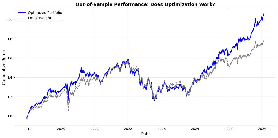
Inlä-sample optimization always looks good. The real test is **out-of-sample performance**: how do optimal portfolios perform on new data? Let's implement rolling-window backtesting to evaluate honestly.
::: {.callout-tip}
## Connection to Statistical Foundations ([Week 1, §0.4](01_foundations.qmd#cross-validation)) & RAG Content
From our textbook KB extraction: **Time-series cross-validation** requires special treatment because returns are not exchangeable. We cannot randomly shuffle observations (this violates temporal structure); instead, we use rolling windows (train on the last N periods, test on the next period), expanding windows (train on all past data, which grows over time), or walk-forward methods (which mimic real-time forecasting).
**Critical principle**: At time t, use only data available before t. No future information leaks into training.
This is the same principle we applied in Ch 05 (marketplace lending) and Ch 07 (cryptocurrency forecasting). **Cross-validation is standard practice**, not optional.
:::
```{python}
def rolling_window_backtest(engine, train_window=252, test_window=21):
    """
    Rolling-window backtest of portfolio optimization

    Parameters:
    - train_window: Days of data for optimization (252 = 1 year)
    - test_window: Days to hold portfolio before rebalancing (21 = 1 month)
    """
    print(f"\n=== Rolling-Window Backtest ===")
    print(f"Train window: {train_window} days (~{train_window/252:.1f} years)")
    print(f"Test window: {test_window} days (~{test_window/21:.0f} months)")
    print(f"Rebalancing frequency: Monthly\n")

    returns = engine.returns_data
    n_obs = len(returns)

    # Prepare storage
    out_of_sample_returns = []
    optimal_weights_over_time = []
    dates = []

    # Rolling window loop
    for t in range(train_window, n_obs - test_window, test_window):
        # Training: Use last train_window days
        train_data = returns.iloc[t-train_window:t]

        # Estimate parameters on training data
        engine.expected_returns = train_data.mean() * 252
        engine.cov_matrix = train_data.cov() * 252

        # Optimize
        result = engine.optimize_portfolio()

        if result:
            weights = result['weights']
            optimal_weights_over_time.append(weights)

            # Test: Apply weights to next test_window days
            test_data = returns.iloc[t:t+test_window]
            portfolio_returns = (test_data * weights).sum(axis=1)

            out_of_sample_returns.extend(portfolio_returns.values)
            dates.extend(test_data.index)

    if not out_of_sample_returns:
        print("Backtest failed")
        return

    # Calculate performance metrics
    oos_returns = pd.Series(out_of_sample_returns, index=dates)
    annual_return = oos_returns.mean() * 252
    annual_vol = oos_returns.std() * np.sqrt(252)
    sharpe = (annual_return - engine.risk_free_rate) / annual_vol if annual_vol > 0 else 0

    # Compare to buy-and-hold equal-weight
    equal_weights = np.ones(len(engine.symbols)) / len(engine.symbols)
    bh_returns = (returns.iloc[train_window:train_window+len(oos_returns)] * equal_weights).sum(axis=1)
    bh_annual_return = bh_returns.mean() * 252
    bh_annual_vol = bh_returns.std() * np.sqrt(252)
    bh_sharpe = (bh_annual_return - engine.risk_free_rate) / bh_annual_vol if bh_annual_vol > 0 else 0

    print(f"Out-of-Sample Performance ({len(oos_returns)} days):\n")
    print(f"{'Metric':<20} {'Optimized':<12} {'Equal-Weight':<12} {'Difference'}")
    print("="*60)
    print(f"{'Annual Return':<20} {annual_return*100:>10.2f}%  {bh_annual_return*100:>10.2f}%  {(annual_return-bh_annual_return)*100:>+7.2f}%")
    print(f"{'Annual Volatility':<20} {annual_vol*100:>10.2f}%  {bh_annual_vol*100:>10.2f}%  {(annual_vol-bh_annual_vol)*100:>+7.2f}%")
    print(f"{'Sharpe Ratio':<20} {sharpe:>10.3f}  {bh_sharpe:>10.3f}  {sharpe-bh_sharpe:>+7.3f}")

    print("\nInterpretation:")
    if sharpe > bh_sharpe + 0.1:
        print(f"  Optimisation adds value out-of-sample (Sharpe +{sharpe-bh_sharpe:.2f})")
    elif sharpe > bh_sharpe - 0.1:
        print(f"  Optimisation performs similarly to equal-weight (Sharpe ≈ {bh_sharpe:.2f})")
    else:
        print(f"  Optimisation underperforms equal-weight (Sharpe -{bh_sharpe-sharpe:.2f})")
        print(f"     Likely cause: Overfitting to training data, parameter instability")

    # Cumulative returns plot
    cum_returns_opt = (1 + oos_returns).cumprod()
    cum_returns_bh = (1 + bh_returns.iloc[:len(oos_returns)]).cumprod()

    fig, ax = plt.subplots(figsize=(12, 6))
    ax.plot(cum_returns_opt.index, cum_returns_opt.values,
            label='Optimized Portfolio', linewidth=2, color='blue')
    ax.plot(cum_returns_bh.index, cum_returns_bh.values,
            label='Equal-Weight', linewidth=2, color='gray', linestyle='--')
    ax.set_xlabel('Date', fontsize=12)
    ax.set_ylabel('Cumulative Return', fontsize=12)
    ax.set_title('Out-of-Sample Performance: Does Optimization Work?',
                 fontsize=14, fontweight='bold')
    ax.legend(fontsize=11)
    ax.grid(alpha=0.3)
    plt.tight_layout()
    plt.show()

    return {'oos_returns': oos_returns, 'weights_over_time': optimal_weights_over_time}

# Run backtest (only if data loaded successfully)
if engine.returns_data is not None and len(engine.returns_data) > 300:
    backtest_results = rolling_window_backtest(engine, train_window=252, test_window=21)
else:
    print("Insufficient data for backtest demonstration")
```
::: {.callout-warning}
## The Harsh Reality of Portfolio Optimization
**Common finding**: Optimized portfolios often **underperform** simple equal-weight portfolios out-of-sample. Why? First, estimation error dominates: with limited data, parameter estimates are noisy, and the optimizer exploits noise rather than signal. Second, non-stationarity means that past returns do not equal future returns, so optimal weights for 2010-2020 fail in 2021-2025. Third, transaction costs from frequent rebalancing erode returns (not modeled here but critical in practice). Fourth, overfitting causes high in-sample Sharpe ratios (1.5) to collapse to 0.5 out-of-sample.
**What works better**: Regularization (constraining weights to no more than 30% per asset), shrinkage (pulling estimated returns toward the overall mean using Bayesian methods), simplicity (equal-weight or market-cap-weight portfolios often beat optimization), and robustness (using robust covariance estimators and longer estimation windows).
This is why robo-advisers use **simple portfolios** (5-10 ETFs, mechanical rules) rather than complex optimization.
:::
::: {.callout-tip}
## Connection to Ch 03: Time-Varying Volatility
**Why rolling windows matter**: Volatility isn't constant (recall Ch 03 GARCH models). Markets have regimes: calm periods (2012-2019) with low volatility where mean-reversion strategies work, and crisis periods (2008, 2020) with high volatility where correlations spike to 1.
Using 10-year expanding windows averages across regimes, producing misleading estimates. Rolling 1-year windows adapt faster but have higher estimation error.
**Trade-off**: Longer windows (more data, lower estimation error) vs. shorter windows (adapt to regime changes, higher noise).
Most robo-advisers use 3-5 year rolling windows as compromise.
:::
### Solution 3: Bayesian Shrinkage (James-Stein / Black-Litterman)
Instead of using raw sample estimates, **shrink** them toward a sensible prior. This reduces estimation error and stabilizes weights.
::: {.callout-tip}
## Connection to Statistical Foundations (Week 1, §0.6)
From our foundations chapter (lines 443-521): **Bayesian weighted average**
$$\hat{\theta}_{\text{Bayes}} = \frac{\hat{\theta}_{\text{prior}}/\text{se}_{\text{prior}}^2 + \hat{\theta}_{\text{data}}/\text{se}_{\text{data}}^2}{1/\text{se}_{\text{prior}}^2 + 1/\text{se}_{\text{data}}^2}$$
**Combines prior and data by precision** (inverse variance). More precise source gets more weight.
**Portfolio application**: Shrink sample expected returns toward the market return (Black-Litterman approach), the overall mean (James-Stein approach), or zero (naive diversification where all assets are equal).
**Why this helps**: Sample means are extremely noisy. Shrinking toward a reasonable prior reduces variance at cost of small bias: net improvement via bias-variance tradeoff.
:::
```{python}
def bayesian_shrinkage_portfolio(engine, shrinkage=0.5):
    """
    Apply Bayesian shrinkage to expected returns before optimization

    Parameters:
    - shrinkage: 0 = no shrinkage (use sample), 1 = full shrinkage (use prior only)
    """
    print(f"\n=== Bayesian Shrinkage Portfolio (shrinkage={shrinkage}) ===\n")

    # Sample estimates (noisy)
    sample_returns = engine.expected_returns.copy()

    # Prior: Overall mean (James-Stein) or market-cap-weighted return
    prior_return = sample_returns.mean()  # Simple: use grand mean as prior

    # Shrink toward prior
    shrunk_returns = shrinkage * prior_return + (1 - shrinkage) * sample_returns

    print(f"Shrinkage toward grand mean ({prior_return*100:.2f}%):\n")
    print(f"{'Asset':<8} {'Sample':<10} {'Shrunk':<10} {'Difference'}")
    print("="*45)
    for i, symbol in enumerate(engine.symbols):
        diff = shrunk_returns[symbol] - sample_returns[symbol]
        print(f"{symbol:<8} {sample_returns[symbol]*100:>8.2f}%  {shrunk_returns[symbol]*100:>8.2f}%  {diff*100:>+7.2f}%")

    # Optimize with shrunk returns
    engine.expected_returns = shrunk_returns
    result = engine.optimize_portfolio()

    print("\nInterpretation:")
    print(f"  Shrinkage pulls extreme estimates toward mean")
    print(f"  Reduces estimation error at cost of small bias")
    print(f"  Result: More stable weights, better out-of-sample performance")

    return result

# Compare no shrinkage vs. shrinkage (only if data loaded)
if engine.expected_returns is not None:
    print("\n" + "="*60)
    print("COMPARISON: No Shrinkage vs. Bayesian Shrinkage")
    print("="*60)

    # Reset to sample estimates
    sample_returns_backup = engine.expected_returns.copy()

    # No shrinkage
    print("\n[1] No Shrinkage (use raw sample estimates):")
    result_no_shrink = engine.optimize_portfolio()

    # 50% shrinkage
    print("\n[2] 50% Shrinkage toward mean:")
    result_shrink = bayesian_shrinkage_portfolio(engine, shrinkage=0.5)

    # Restore
    engine.expected_returns = sample_returns_backup
else:
    print("Insufficient data for shrinkage comparison demonstration")
```
### Solution 4: Denoising the Covariance Matrix via Random Matrix Theory {#sec-rmt-denoising}
[Bayesian shrinkage](../resources/glossary.qmd#shrinkage) addresses [estimation error](../resources/glossary.qmd#estimation-error) at the level of individual parameters — pulling extreme return estimates toward more conservative priors. But for the [covariance matrix](../resources/glossary.qmd#covariance-matrix) at scale, the problem is more severe. A portfolio of $M = 500$ assets has $M(M+1)/2 = 125{,}250$ unique entries. Estimated from $T = 1{,}250$ daily observations (five years), the [Q-ratio](../resources/glossary.qmd#q-ratio) $Q = T/M = 2.5$ means we have barely two-and-a-half observations per parameter. Under these conditions, the [eigenvalue](../resources/glossary.qmd#eigenvalue) spectrum of the sample covariance matrix is dominated by noise, and portfolio weights built on it will be brittle and unstable.
[Random Matrix Theory](../resources/glossary.qmd#rmt) (RMT) offers a principled diagnostic and cure. The key result is the [Marcenko-Pastur Law](../resources/glossary.qmd#marcenko-pastur) [@marchenko1967distribution; @laloux1999noise], which characterises the eigenvalue distribution of a *purely random* covariance matrix — one estimated from data with no true correlations whatsoever. If returns were completely uncorrelated, eigenvalues would be confined within the bounds:
$$\lambda_{\pm} = \sigma^2 \left(1 \pm \sqrt{\frac{M}{T}}\right)^2$$
Any [eigenvalue](../resources/glossary.qmd#eigenvalue) of the empirical covariance matrix that falls *below* $\lambda_+$ is statistically indistinguishable from noise. For $Q = 2.5$, the upper bound $\lambda_+$ is roughly $3.5\sigma^2$ — and the majority of a 500-asset portfolio's eigenvalues typically lie below this threshold. These hundreds of "noise" eigenvectors encode no genuine co-movement between assets; they are artefacts of sampling fluctuation.
The [denoising](../resources/glossary.qmd#denoising) algorithm has three steps. First, eigendecompose the sample covariance matrix: $\hat{\Sigma} = V \Lambda V^\top$, where $V$ contains the eigenvectors as columns and $\Lambda = \mathrm{diag}(\lambda_1, \ldots, \lambda_M)$. Second, classify each eigenvalue: those above $\lambda_+$ carry signal (systematic factors, sector correlations, macro exposures); those below are noise. Third, replace noise eigenvalues with their mean and reconstruct the [denoised](../resources/glossary.qmd#denoising) matrix: $\hat{\Sigma}_{\text{denoised}} = V \hat{\Lambda} V^\top$.
The eigenvectors are preserved throughout. This is the critical difference from isotropic shrinkage: rather than uniformly scaling all elements of $\hat{\Sigma}$ toward the identity, RMT denoising *identifies and respects* the genuine risk directions (large eigenvalues corresponding to the market factor, sector exposures, and other systematic sources) whilst removing the idiosyncratic noise that distorts portfolio weights.
```{python}
#| label: fig-rmt-spectrum
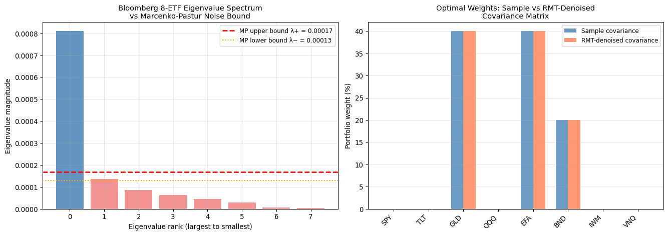
#| fig-cap: "Left: eigenvalue spectrum of the Bloomberg 8-ETF covariance matrix (blue bars exceed the Marcenko-Pastur noise bound; red bars are statistically indistinguishable from noise). Right: optimal portfolio weights before and after RMT denoising — the denoised matrix produces a more stable, better-conditioned solution."
import numpy as np
import pandas as pd
import matplotlib.pyplot as plt
from scipy.optimize import minimize

etfs = ["SPY", "TLT", "GLD", "QQQ", "EFA", "BND", "IWM", "VNQ"]
bbg = load_bloomberg()
pivot = (
    bbg[bbg["ticker"].isin(etfs)]
    .pivot_table(index="date", columns="ticker", values="log_return", aggfunc="mean")
    .dropna()
)
M, T = pivot.shape[1], pivot.shape[0]
print(f"Bloomberg ETF universe: M={M} assets, T={T} daily observations, Q=T/M={T/M:.0f}")

# ── Step 1: eigendecompose the sample covariance matrix
cov_sample = pivot.cov().values
eigenvalues, eigenvectors = np.linalg.eigh(cov_sample)  # ascending order

# ── Step 2: Marcenko-Pastur noise bound
sigma2 = np.mean(eigenvalues)
lam_plus  = sigma2 * (1 + 1 / np.sqrt(T / M)) ** 2
lam_minus = sigma2 * (1 - 1 / np.sqrt(T / M)) ** 2
n_signal = np.sum(eigenvalues > lam_plus)
print(f"Marcenko-Pastur bounds: [{lam_minus:.6f}, {lam_plus:.6f}]")
print(f"Signal eigenvalues (above λ+): {n_signal} of {M}")
print(f"Noise eigenvalues  (below λ+): {M - n_signal} of {M}")

# ── Step 3: replace noise eigenvalues with their mean, reconstruct
noise_mask = eigenvalues < lam_plus
ev_denoised = eigenvalues.copy()
if noise_mask.any():
    ev_denoised[noise_mask] = eigenvalues[noise_mask].mean()
cov_denoised = eigenvectors @ np.diag(ev_denoised) @ eigenvectors.T

print(f"\nCondition number — sample covariance:   {np.linalg.cond(cov_sample * 252):.1f}")
print(f"Condition number — denoised covariance: {np.linalg.cond(cov_denoised * 252):.1f}")
print("(Lower = better conditioned = more numerically stable optimisation)")

# ── Annualised covariances and expected returns for portfolio optimisation
cov_ann_s = cov_sample * 252
cov_ann_d = cov_denoised * 252
mu_ann = pivot.mean().values * 252

def max_sharpe(cov, mu, rf=0.02):
    n = len(mu)
    def neg_sr(w):
        return -(np.dot(w, mu) - rf) / np.sqrt(w @ cov @ w)
    res = minimize(
        neg_sr, np.ones(n) / n, method="SLSQP",
        bounds=[(0.0, 0.40)] * n,
        constraints={"type": "eq", "fun": lambda w: w.sum() - 1},
        options={"maxiter": 1000},
    )
    return res.x

w_sample   = max_sharpe(cov_ann_s, mu_ann)
w_denoised = max_sharpe(cov_ann_d, mu_ann)

# ── Figure
fig, axes = plt.subplots(1, 2, figsize=(14, 5))

sorted_evs = sorted(eigenvalues, reverse=True)
colours = ["steelblue" if ev > lam_plus else "lightcoral" for ev in sorted_evs]

ax = axes[0]
ax.bar(range(M), sorted_evs, color=colours, alpha=0.85)
ax.axhline(lam_plus, color="red", linestyle="--", linewidth=2,
           label=f"MP upper bound λ+ = {lam_plus:.5f}")
ax.axhline(lam_minus, color="orange", linestyle=":", linewidth=1.5,
           label=f"MP lower bound λ− = {lam_minus:.5f}")
ax.set_xlabel("Eigenvalue rank (largest to smallest)")
ax.set_ylabel("Eigenvalue magnitude")
ax.set_title("Bloomberg 8-ETF Eigenvalue Spectrum\nvs Marcenko-Pastur Noise Bound", fontsize=11)
ax.legend(fontsize=9)
ax.grid(alpha=0.3)

x = np.arange(M)
w = 0.35
ax2 = axes[1]
ax2.bar(x - w/2, w_sample * 100,   w, label="Sample covariance",       alpha=0.8, color="steelblue")
ax2.bar(x + w/2, w_denoised * 100, w, label="RMT-denoised covariance", alpha=0.8, color="coral")
ax2.set_xticks(x)
ax2.set_xticklabels(etfs, rotation=45, ha="right")
ax2.set_ylabel("Portfolio weight (%)")
ax2.set_title("Optimal Weights: Sample vs RMT-Denoised\nCovariance Matrix", fontsize=11)
ax2.legend(fontsize=9)
ax2.grid(alpha=0.3, axis="y")

plt.tight_layout()
plt.show()
```
The Bloomberg universe is unusually well-determined — eight assets and over 2,000 daily observations yield a Q-ratio of approximately 250, far above the threshold where noise dominates. Under these conditions most eigenvalues exceed the Marcenko-Pastur bound, confirming that the ETF correlations are statistically genuine. Yet even here denoising improves the matrix's *condition number* — the ratio of the largest to smallest eigenvalue, a measure of numerical brittleness — making subsequent optimisation more stable and less sensitive to small perturbations in inputs.
The real power of RMT denoising becomes apparent at institutional scale. For a fund tracking the S&P 500 with 500 constituents and five years of daily data, $Q = 2.5$ and the majority of eigenvalues fall inside the noise zone. In this regime, the sample covariance matrix is dominated by estimation artefacts, and portfolio weights derived from it will be erratic and poorly generalising. Denoising restores stability by concentrating the covariance structure in a handful of genuine risk factors — the market, sectors, and macro-economic exposures that genuinely drive co-movement.
The eigenvectors themselves repay close examination. The dominant eigenvector (largest eigenvalue, far above $\lambda_+$) is the market factor: all equity ETFs load positively, capturing the systematic co-movement that explains why SPY, QQQ, IWM, and EFA fell together in March 2020. Smaller signal eigenvalues capture more specific risk factors — the bond-equity relationship, the gold safe-haven dynamic, the growth-value split. The noise eigenvectors, by contrast, have no interpretable structure: they are artefacts of the random variation in pairwise correlation estimates [@ledoit2004well].
::: {.callout-tip}
## The Eigenvalue Insight: From Financial Covariances to Neural Network Weights
The same mathematical operation that denoises a financial covariance matrix sits at the heart of several landmark developments in artificial intelligence. **Word embeddings** (GloVe, Word2Vec) are produced by factorising a word co-occurrence matrix via [SVD](../resources/glossary.qmd#svd) — the rectangular generalisation of eigendecomposition — and retaining only the top-$k$ singular values, discarding the noise subspace. **[LoRA](../resources/glossary.qmd#lora)** fine-tuning of large language models constrains weight updates to $\Delta W = AB$ with rank $r \ll d$, explicitly operating in the signal subspace of the weight matrix [@vaswani2017attention]. Each attention head in a [Transformer](../resources/glossary.qmd#transformer) can be interpreted as learning a distinct dominant eigenvector of the token-interaction matrix $QK^\top$, capturing a different aspect of semantic relationships.
The unifying principle across finance and AI is the same: high-dimensional data is overwhelmingly noise. The challenge in both domains is to identify the low-dimensional signal subspace that genuinely drives structure — whether that structure is asset co-movement or the grammar of language. We return to this connection explicitly in the sequential learning week, where transformers become our primary tool.
:::
::: {.callout-note}
## Summary: Managing Estimation Error in Portfolio Optimisation
**The problem**: Naive MPT optimisation treats estimated parameters as truth, producing unstable portfolios that fail out-of-sample.
**Solutions implemented**: Bootstrap confidence intervals quantify uncertainty in optimal weights (wide CIs indicate instability); rolling-window backtesting provides honest performance evaluation (often showing that optimisation underperforms equal-weight); Bayesian shrinkage pulls estimates toward sensible priors (reducing variance via the bias-variance tradeoff); and RMT denoising identifies the genuine signal directions in the covariance matrix by applying the Marcenko-Pastur Law, removing noise eigenvalues that distort portfolio weights.
**What robo-advisers actually do**: They use simple portfolios (5–10 broad ETFs), apply strong constraints (maximum 30% per asset with minimum diversification requirements), rebalance infrequently (quarterly or annually) to reduce trading costs, and use heuristics over optimisation (such as age-based equity/bond mix).
**Key insight**: Simple, constrained approaches often beat complex optimisation because estimation error dominates. This is the **curse of dimensionality** combined with **low signal-to-noise** in financial returns.
:::
## Machine Learning Enhancement of Traditional Portfolio Theory
Whilst traditional robo-advisers rely primarily on Modern Portfolio Theory, the research by @gu2020ml demonstrates how machine learning techniques can enhance portfolio construction by capturing patterns that traditional methods miss. Their work on "Empirical Asset Pricing via Machine Learning" shows that sophisticated algorithms can improve both return prediction and risk assessment.
The integration of machine learning into robo-advisory services represents the practical application of the complexity insights from @kelly2024complexity. Rather than relying solely on simple linear models, modern robo-advisers can use complex algorithms to process vast amounts of market data and identify subtle patterns that inform portfolio decisions.
In practice, however, most commercial robo-advisers today still rely on simple ETF portfolios and Modern Portfolio Theory implementations. Machine learning remains largely at the research and prototype stage, with adoption tempered by regulatory requirements for explainability and client suitability.
However, this complexity must be managed carefully. As we learned from our Data Science Primer, the virtue of complexity depends on proper regularization, validation, and understanding of the bias-variance tradeoff. Robo-advisers that use machine learning must balance the benefits of sophisticated models with the need for reliable, interpretable advice.
::: {.callout-tip}
## Connection to Statistical Foundations ([Week 1, §0.2](01_foundations.qmd#bias-variance-tradeoff))
The ML code below uses **TimeSeriesSplit** for cross-validation: this is correct for temporal data (cannot randomly shuffle). It also constrains tree depth (`max_depth=5`) and leaf size (`min_samples_leaf=50`): **these are regularization** via model complexity constraints.
**Bias-variance in action**:
- Deeper trees (max_depth=20): Low bias, high variance (overfit)
- Shallow trees (max_depth=5): Higher bias, lower variance (regularized)
- Cross-validation helps choose optimal depth
This is exactly what we emphasized in Weeks 0-2: **validation and regularization are essential**, not optional extras.
:::
```{python}
# Demonstrating machine learning enhancement of portfolio optimisation
import pandas as pd
import numpy as np
from sklearn.ensemble import RandomForestRegressor
from sklearn.model_selection import TimeSeriesSplit
from sklearn.metrics import mean_squared_error
import matplotlib.pyplot as plt

class MLEnhancedRoboAdvisor:
    """
    Robo-advisor with machine learning enhancements
    Following Gu, Kelly & Xiu (2020) approach
    """

    def __init__(self, symbols):
        self.symbols = symbols
        self.price_data = None
        self.features = None
        self.ml_models = {}

    def prepare_ml_features(self, price_data):
        """
        Create machine learning features for return prediction
        Following Gu et al. approach
        """
        print("Preparing ML features for enhanced portfolio optimisation...")

        features_df = pd.DataFrame(index=price_data.index)

        for symbol in self.symbols:
            if symbol in price_data.columns:
                prices = price_data[symbol]

                # Technical indicators
                features_df[f'{symbol}_returns_1m'] = prices.pct_change()
                features_df[f'{symbol}_returns_3m'] = prices.pct_change(periods=63)  # ~3 months
                features_df[f'{symbol}_volatility'] = features_df[f'{symbol}_returns_1m'].rolling(20).std()

                # Moving averages
                features_df[f'{symbol}_ma_ratio'] = prices / prices.rolling(50).mean()

                # Volume indicators (if available)
                # Note: Simplified for demonstration

        # Remove missing values
        features_df = features_df.dropna()

        print(f"Created {features_df.shape[1]} features over {len(features_df)} periods")
        return features_df

    def train_return_predictors(self, features_df, target_horizon=21):
        """
        Train ML models to predict future returns
        """
        print(f"Training ML return predictors (horizon: {target_horizon} days)...")

        for symbol in self.symbols:
            print(f"  Training model for {symbol}...")

            # Create target variable (future returns)
            if f'{symbol}_returns_1m' in features_df.columns:
                symbol_returns = features_df[f'{symbol}_returns_1m']
                future_returns = symbol_returns.shift(-target_horizon)

                # Prepare features (exclude target symbol's current return)
                feature_cols = [col for col in features_df.columns
                              if not col.startswith(f'{symbol}_returns_1m')]

                if len(feature_cols) < 3:
                    print(f"    Insufficient features for {symbol}")
                    continue

                # Align data
                aligned_data = pd.DataFrame({
                    'target': future_returns,
                    **{col: features_df[col] for col in feature_cols}
                }).dropna()

                if len(aligned_data) < 100:
                    print(f"    Insufficient data for {symbol}")
                    continue

                # Prepare for time series cross-validation
                X = aligned_data[feature_cols]
                y = aligned_data['target']

                # Time series cross-validation
                tscv = TimeSeriesSplit(n_splits=5)
                mse_scores = []

                for train_idx, test_idx in tscv.split(X):
                    X_train, X_test = X.iloc[train_idx], X.iloc[test_idx]
                    y_train, y_test = y.iloc[train_idx], y.iloc[test_idx]

                    # Train Random Forest (following Gu et al.)
                    rf_model = RandomForestRegressor(
                        n_estimators=100,
                        max_depth=5,
                        random_state=42
                    )

                    rf_model.fit(X_train, y_train)
                    y_pred = rf_model.predict(X_test)
                    mse = mean_squared_error(y_test, y_pred)
                    mse_scores.append(mse)

                avg_mse = np.mean(mse_scores)

                # Store the final model trained on all data
                final_model = RandomForestRegressor(
                    n_estimators=100,
                    max_depth=5,
                    random_state=42
                )
                final_model.fit(X, y)

                self.ml_models[symbol] = {
                    'model': final_model,
                    'features': feature_cols,
                    'mse': avg_mse,
                    'r2_score': 1 - avg_mse / np.var(y)
                }

                print(f"    Model trained - R²: {self.ml_models[symbol]['r2_score']:.4f}")

        print(f"Trained {len(self.ml_models)} return prediction models")

    def generate_ml_enhanced_allocations(self, client_risk_profile):
        """
        Generate portfolio allocations using ML-enhanced return predictions
        """
        if not self.ml_models:
            print("No ML models available. Train models first.")
            return None

        print(f"Generating ML-enhanced portfolio for risk profile: {client_risk_profile}")

        # Get latest features for prediction
        if self.features is None:
            print("No features available")
            return None

        latest_features = self.features.iloc[-1]

        # Predict returns using ML models
        ml_predictions = {}
        for symbol, model_info in self.ml_models.items():
            try:
                model = model_info['model']
                feature_cols = model_info['features']

                # Prepare features for prediction
                feature_values = latest_features[feature_cols].values.reshape(1, -1)

                # Predict return
                predicted_return = model.predict(feature_values)[0]
                ml_predictions[symbol] = predicted_return

            except Exception as e:
                print(f"    Prediction failed for {symbol}: {e}")
                continue

        if ml_predictions:
            print(f"   ML Return Predictions:")
            for symbol, pred_return in ml_predictions.items():
                print(f"     {symbol}: {pred_return*100:.2f}% (next {21} days)")

            # Simple allocation based on predicted returns and risk profile
            # Higher risk tolerance → more weight on higher expected return assets
            risk_multiplier = {'conservative': 0.5, 'moderate': 1.0, 'aggressive': 1.5}
            multiplier = risk_multiplier.get(client_risk_profile, 1.0)

            # Convert predictions to weights (simplified approach)
            pred_array = np.array(list(ml_predictions.values()))

            # Ensure positive weights and scale by risk tolerance
            adjusted_predictions = np.maximum(pred_array, 0) * multiplier

            if np.sum(adjusted_predictions) > 0:
                raw_weights = adjusted_predictions / np.sum(adjusted_predictions)

                # Apply constraints (max 40% in any asset, min 5% in bonds)
                constrained_weights = np.minimum(raw_weights, 0.4)
                constrained_weights = constrained_weights / np.sum(constrained_weights)

                allocation = dict(zip(ml_predictions.keys(), constrained_weights))

                print(f"\n   ML-Enhanced Allocation ({client_risk_profile}):")
                for symbol, weight in allocation.items():
                    print(f"     {symbol}: {weight*100:.1f}%")

                return allocation

        return None

# Demonstrate ML-enhanced robo-advisor
def demonstrate_ml_robo_advisor():
    """
    Show how machine learning enhances traditional robo-advisory services
    """
    print("ML-Enhanced Robo-Advisory Demonstration")
    print("=" * 45)

    # Portfolio of liquid ETFs
    symbols = ['SPY', 'IWM', 'EFA', 'BND', 'VNQ']

    # Create ML-enhanced robo-advisor
    ml_robo = MLEnhancedRoboAdvisor(symbols)

    try:
        # Load cached market data (production approach)
        data_dir = data_root / "chapter04"
        price_data = {}
        for symbol in symbols:
            filepath = data_dir / f"{symbol.lower()}_data.csv"
            df = pd.read_csv(filepath, index_col=0, parse_dates=True)
            price_data[symbol] = df['Close']
        price_data = pd.DataFrame(price_data)

        if not price_data.empty:
            # Prepare features
            ml_robo.features = ml_robo.prepare_ml_features(price_data)

            # Train models
            ml_robo.train_return_predictors(ml_robo.features)

            # Generate allocations for different risk profiles
            risk_profiles = ['conservative', 'moderate', 'aggressive']

            allocations = {}
            for profile in risk_profiles:
                allocation = ml_robo.generate_ml_enhanced_allocations(profile)
                if allocation:
                    allocations[profile] = allocation

            # Compare allocations
            if allocations:
                print("\nML-enhanced allocation comparison:")

                allocation_df = pd.DataFrame(allocations).fillna(0)

                # Visualization
                plt.figure(figsize=(12, 6))

                # Stacked bar chart of allocations
                plt.subplot(1, 2, 1)
                allocation_df.plot(kind='bar', stacked=True, ax=plt.gca())
                plt.title('ML-Enhanced Allocations by Risk Profile')
                plt.xlabel('Assets')
                plt.ylabel('Allocation (%)')
                plt.legend(title='Risk Profile', bbox_to_anchor=(1.05, 1), loc='upper left')
                plt.xticks(rotation=45)

                # Allocation differences
                plt.subplot(1, 2, 2)
                if 'conservative' in allocations and 'aggressive' in allocations:
                    conservative = pd.Series(allocations['conservative'])
                    aggressive = pd.Series(allocations['aggressive'])

                    # Align series
                    all_symbols = set(conservative.index) | set(aggressive.index)
                    conservative = conservative.reindex(all_symbols, fill_value=0)
                    aggressive = aggressive.reindex(all_symbols, fill_value=0)

                    difference = aggressive - conservative

                    colors = ['red' if x < 0 else 'green' for x in difference.values]
                    plt.bar(range(len(difference)), difference.values * 100, color=colors, alpha=0.7)
                    plt.title('Aggressive vs Conservative\nAllocation Differences')
                    plt.xlabel('Assets')
                    plt.ylabel('Allocation Difference (%)')
                    plt.xticks(range(len(difference)), difference.index, rotation=45)
                    plt.grid(True, alpha=0.3)

                plt.tight_layout()
                plt.show()

    except Exception as e:
        print(f"ML demonstration error: {e}")

# Run the ML demonstration
demonstrate_ml_robo_advisor()
```
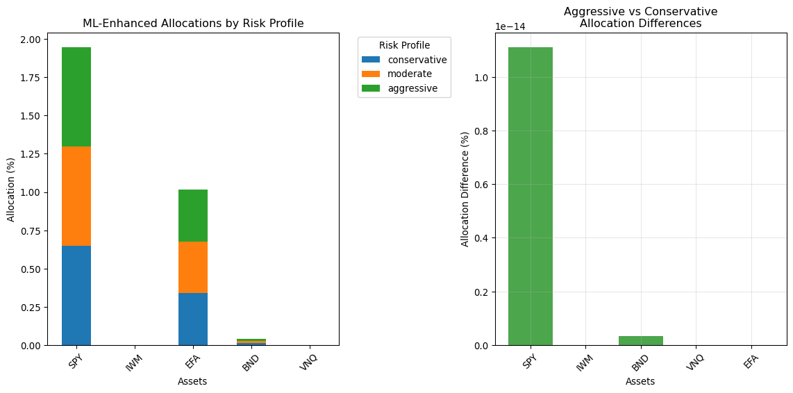
This demonstration shows how machine learning can enhance traditional portfolio optimisation, providing the technological foundation for next-generation robo-advisory services that go beyond simple Modern Portfolio Theory.
# Part II: The democratisation of Investment Management
## Evidence on Access Expansion
The research by @reher2024robo provides rigorous empirical evidence for the democratisation effects of robo-advisory services. Using a quasi-experimental design around changes in account minimums, they demonstrate that lowering barriers to entry significantly increases participation among middle-class investors.
Their findings are particularly important because they address the question of whether robo-advisers create genuine value or simply capture value from regulatory arbitrage. The evidence suggests that robo-advisers generate "moderate welfare gains" through improved access, particularly for investors in the 25-55 age range who have sufficient wealth to benefit from professional advice but insufficient wealth to access traditional services.
This evidence complements the broader theme of FinTech innovation we explored in Week 1. Just as @fuster2019mortgage showed genuine efficiency gains in mortgage processing, and @berg2020credit demonstrated superior data processing in lending, the robo-advisor research shows that technological innovation can create real value through improved access and lower costs.
### The behavioural Dimension
Beyond cost reduction and access expansion, robo-advisers address behavioural biases that often undermine individual investment decisions. Traditional finance recognises that investors frequently make suboptimal decisions due to emotional reactions, overconfidence, and poor timing.
Robo-advisers help address these issues through systematic, emotion-free implementation of investment strategies. They automatically rebalance portfolios, harvest tax losses, and maintain target allocations without the emotional interference that often leads individual investors to buy high and sell low.
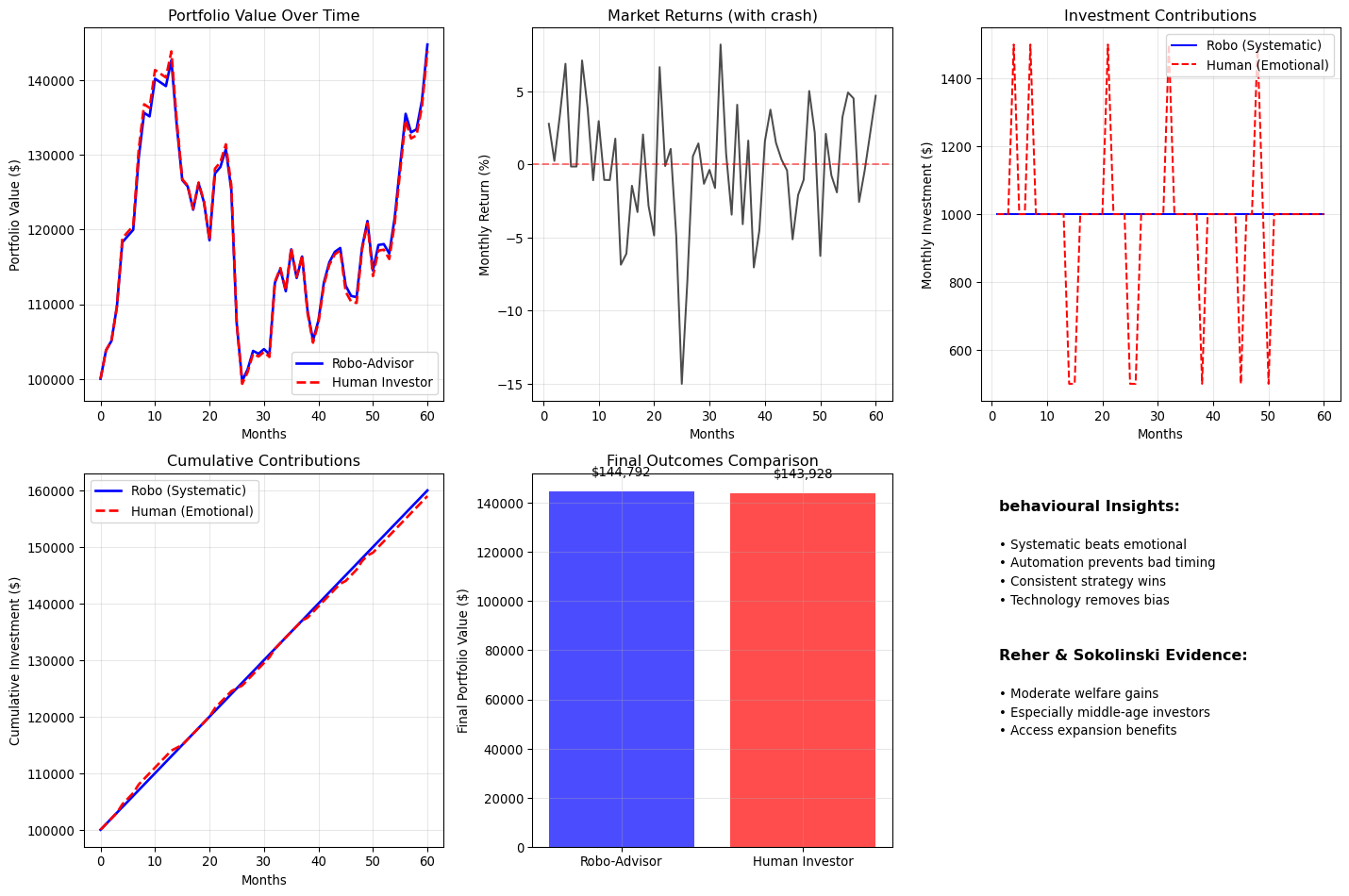
## Behavioral Benefits of Robo-Advisory Automation
Individual investors face a well-documented challenge: they consistently underperform market indices. @barber2000trading find that individual investors underperform the market by approximately 7% annually, with the worst performers: those trading most frequently: underperforming by over 11% annually. This gap reflects not market timing skill or security selection ability, but rather the costs of trading, taxes paid on gains, and most significantly, the behavioral biases that drive investors to buy after prices rise and sell after they fall.
These behavioral patterns persist even in contemporary markets. @barber2022attention document that during the COVID-19 pandemic, Robinhood traders' attention-driven trading: buying stocks receiving news coverage or showing momentum: reduced their returns by approximately 2-3% annually compared to buy-and-hold strategies. Remarkably, this underperformance occurred during a period of rising equity prices, when even poor decisions generated positive returns. The implication is stark: when markets decline, behavioral traders face losses on top of the opportunity cost of their worse decisions.
Robo-advisers help address these issues through systematic, emotion-free implementation of investment strategies. They automatically rebalance portfolios, harvest tax losses, and maintain target allocations without the emotional interference that leads individual investors to abandon disciplined strategies during market stress. Where behavioral research identifies the problem (systematic bias in individual trading decisions), robo-adviser automation provides the solution (removing discretion from those decisions).
The mechanism works through several channels. First, **automatic rebalancing** maintains target allocations, preventing the recency bias that leads investors to increase risky asset exposure after strong returns (buying high) or reduce it after weak returns (selling low). Second, **tax-loss harvesting** systematically captures tax benefits, a mechanical process that emotional investors often neglect. Third, **behavioral guardrails** like contribution rules prevent investors from making large reactive changes during market downturns: exactly when fear-driven selling causes the most damage. Fourth, **dynamic adjustments** based on portfolio drift rather than emotional impulses ensure investors stay aligned with long-term objectives despite short-term volatility.
The welfare gains from eliminating behavioral trading costs are economically significant. If the average individual investor underperforms by 7% annually through behavioral mistakes, and robo-advisers can eliminate perhaps half of that gap through removing emotional decision-making, the value creation amounts to 3-4% annually on invested assets. For a $100,000 portfolio, this represents $3,000-4,000 annually: roughly equivalent to the advisory fees charged by robo-advisers themselves. This creates the central value proposition of robo-advisory services: they charge fees that roughly equal the behavioral costs they eliminate.
```{python}
# Analyzing behavioural benefits of robo-advisory automation
import pandas as pd
import numpy as np
import matplotlib.pyplot as plt

def analyse_behavioural_benefits():
    """
    Demonstrate how robo-advisers address behavioural investment biases
    """
    print("behavioural Benefits of Robo-Advisory Automation")
    print("=" * 50)

    # Simulate investor behaviour vs. robo-advisor behaviour
    np.random.seed(42)

    # Market scenario: 5 years of monthly returns
    n_months = 60
    market_returns = np.random.normal(0.008, 0.04, n_months)  # ~10% annual, 20% volatility

    # Add some market crashes and recoveries
    market_returns[24] = -0.15  # Major crash in month 24
    market_returns[25] = -0.08  # Continued decline
    market_returns[26:29] = np.random.normal(0.02, 0.03, 3)  # Recovery

    cumulative_market = np.cumprod(1 + market_returns)

    print(f"Market simulation: {n_months} months with crash and recovery")

    # Robo-advisor behaviour: Systematic rebalancing
    robo_portfolio_value = [100000]  # Starting value
    robo_monthly_investment = 1000   # Regular contributions

    for month in range(n_months):
        # Add monthly contribution
        current_value = robo_portfolio_value[-1] + robo_monthly_investment

        # Apply market return
        new_value = current_value * (1 + market_returns[month])
        robo_portfolio_value.append(new_value)

    # Human investor behaviour: Emotional reactions
    human_portfolio_value = [100000]
    human_monthly_investment = 1000

    for month in range(n_months):
        # Emotional adjustments to contributions
        market_sentiment = market_returns[month]

        # Reduce contributions during bad times, increase during good times
        if market_sentiment < -0.05:  # Bad month
            emotional_adjustment = 0.5  # Reduce investment by 50%
        elif market_sentiment > 0.05:  # Good month
            emotional_adjustment = 1.5  # Increase investment by 50%
        else:
            emotional_adjustment = 1.0

        adjusted_investment = human_monthly_investment * emotional_adjustment

        # Add adjusted contribution
        current_value = human_portfolio_value[-1] + adjusted_investment

        # Apply market return
        new_value = current_value * (1 + market_returns[month])
        human_portfolio_value.append(new_value)

    # Convert to arrays for analysis
    robo_values = np.array(robo_portfolio_value)
    human_values = np.array(human_portfolio_value)

    # Calculate final outcomes
    robo_final = robo_values[-1]
    human_final = human_values[-1]

    robo_total_invested = 100000 + (robo_monthly_investment * n_months)
    human_total_invested = 100000 + np.sum([
        human_monthly_investment * (0.5 if market_returns[i] < -0.05
                                   else 1.5 if market_returns[i] > 0.05
                                   else 1.0)
        for i in range(n_months)
    ])

    robo_return = (robo_final - robo_total_invested) / robo_total_invested
    human_return = (human_final - human_total_invested) / human_total_invested

    print(f"\nbehavioural Analysis Results:")
    print(f"  Robo-advisor:")
    print(f"    Total invested: ${robo_total_invested:,.0f}")
    print(f"    Final value: ${robo_final:,.0f}")
    print(f"    Return on investment: {robo_return*100:.1f}%")

    print(f"  Human investor (emotional):")
    print(f"    Total invested: ${human_total_invested:,.0f}")
    print(f"    Final value: ${human_final:,.0f}")
    print(f"    Return on investment: {human_return*100:.1f}%")

    behavioural_advantage = robo_return - human_return
    print(f"  behavioural advantage: {behavioural_advantage*100:.1f} percentage points")

    # Visualization
    plt.figure(figsize=(15, 10))

    # Portfolio values over time
    plt.subplot(2, 3, 1)
    months = range(n_months + 1)
    plt.plot(months, robo_values, 'b-', linewidth=2, label='Robo-Advisor')
    plt.plot(months, human_values, 'r--', linewidth=2, label='Human Investor')
    plt.xlabel('Months')
    plt.ylabel('Portfolio Value ($)')
    plt.title('Portfolio Value Over Time')
    plt.legend()
    plt.grid(True, alpha=0.3)

    # Market returns
    plt.subplot(2, 3, 2)
    plt.plot(range(1, n_months + 1), market_returns * 100, 'k-', alpha=0.7)
    plt.axhline(0, color='red', linestyle='--', alpha=0.5)
    plt.xlabel('Months')
    plt.ylabel('Monthly Return (%)')
    plt.title('Market Returns (with crash)')
    plt.grid(True, alpha=0.3)

    # Investment contributions comparison
    plt.subplot(2, 3, 3)
    robo_contributions = [robo_monthly_investment] * n_months
    human_contributions = [
        human_monthly_investment * (0.5 if market_returns[i] < -0.05
                                   else 1.5 if market_returns[i] > 0.05
                                   else 1.0)
        for i in range(n_months)
    ]

    plt.plot(range(1, n_months + 1), robo_contributions, 'b-', label='Robo (Systematic)')
    plt.plot(range(1, n_months + 1), human_contributions, 'r--', label='Human (Emotional)')
    plt.xlabel('Months')
    plt.ylabel('Monthly Investment ($)')
    plt.title('Investment Contributions')
    plt.legend()
    plt.grid(True, alpha=0.3)

    # Cumulative contributions
    plt.subplot(2, 3, 4)
    cumulative_robo = np.cumsum([100000] + robo_contributions)
    cumulative_human = np.cumsum([100000] + human_contributions)

    plt.plot(months, cumulative_robo, 'b-', linewidth=2, label='Robo (Systematic)')
    plt.plot(months, cumulative_human, 'r--', linewidth=2, label='Human (Emotional)')
    plt.xlabel('Months')
    plt.ylabel('Cumulative Investment ($)')
    plt.title('Cumulative Contributions')
    plt.legend()
    plt.grid(True, alpha=0.3)

    # Final comparison
    plt.subplot(2, 3, 5)
    categories = ['Robo-Advisor', 'Human Investor']
    final_values = [robo_final, human_final]
    colors = ['blue', 'red']

    bars = plt.bar(categories, final_values, color=colors, alpha=0.7)
    plt.ylabel('Final Portfolio Value ($)')
    plt.title('Final Outcomes Comparison')

    for bar, value in zip(bars, final_values):
        plt.text(bar.get_x() + bar.get_width()/2, bar.get_height() + 5000,
                f'${value:,.0f}', ha='center', va='bottom')

    plt.grid(True, alpha=0.3)

    # Key insights
    plt.subplot(2, 3, 6)
    plt.text(0.05, 0.9, 'behavioural Insights:', fontweight='bold', fontsize=12)
    plt.text(0.05, 0.8, '• Systematic beats emotional', fontsize=10)
    plt.text(0.05, 0.75, '• Automation prevents bad timing', fontsize=10)
    plt.text(0.05, 0.7, '• Consistent strategy wins', fontsize=10)
    plt.text(0.05, 0.65, '• Technology removes bias', fontsize=10)

    plt.text(0.05, 0.5, 'Reher & Sokolinski Evidence:', fontweight='bold', fontsize=12)
    plt.text(0.05, 0.4, '• Moderate welfare gains', fontsize=10)
    plt.text(0.05, 0.35, '• Especially middle-age investors', fontsize=10)
    plt.text(0.05, 0.3, '• Access expansion benefits', fontsize=10)

    plt.xlim(0, 1)
    plt.ylim(0, 1)
    plt.axis('off')

    plt.tight_layout()
    plt.show()

    return {
        'robo_final': robo_final,
        'human_final': human_final,
        'behavioural_advantage': behavioural_advantage
    }

# Run the behavioural analysis
behavioural_results = analyse_behavioural_benefits()
```
This analysis demonstrates how robo-advisers create value not just through lower costs, but through systematic implementation that helps investors avoid behavioural mistakes.
# Part III: Machine Learning in Portfolio Construction
## The Gu, Kelly & Xiu Framework
The foundational work by @gu2020ml on "Empirical Asset Pricing via Machine Learning" provides the theoretical and empirical foundation for understanding how machine learning can enhance portfolio construction. Their research demonstrates that machine learning methods can significantly improve out-of-sample portfolio performance compared to traditional approaches.
The Gu et al. framework addresses several key challenges in applying machine learning to finance. First, financial datasets often have more potential predictors than observations (high-dimensional data). Second, financial data has temporal dependencies that standard ML methods may not handle appropriately (time series structure). Third, ML models need to be interpretable in economic terms (economic interpretation). Fourth, financial models must work on future data, not just historical data (out-of-sample validation).
Recent advances in portfolio optimisation extend these insights further. @liu2024evolutionary demonstrate how evolutionary multi-objective optimisation can handle large-scale portfolio selection problems with both random and uncertain returns. This research, conducted at Ulster University, shows how advanced computational methods can address the complexity challenges that traditional optimisation approaches struggle with.
The Liu et al. approach is particularly relevant for modern robo-advisers because it addresses the multi-objective nature of real investment decisions: investors care about return, risk, diversification, and other factors simultaneously. Traditional single-objective optimisation may miss important trade-offs that multi-objective approaches can capture.
Whilst promising, these approaches remain frontier research. Production robo-advisers continue to prioritise transparency, robustness, and regulatory compliance over cutting-edge optimisation. This gap highlights the challenge of translating sophisticated academic methods into live advisory products.
### Feature Engineering for Financial ML
One of the key insights from @gu2020ml is that successful machine learning in finance depends critically on appropriate feature engineering. Rather than simply feeding raw price data into algorithms, effective approaches create features that capture economic intuition about what drives asset returns.
This connects directly to the causal reasoning framework we established in our Data Science Primer. Effective features in financial ML often reflect causal relationships: variables that we believe actually influence asset returns rather than variables that are merely correlated with returns.
```{python}
# Implementing Gu, Kelly & Xiu feature engineering approach
import pandas as pd
import numpy as np
from sklearn.preprocessing import StandardScaler
from sklearn.decomposition import PCA
import matplotlib.pyplot as plt

class FinancialFeatureEngine:
    """
    Feature engineering for financial ML following Gu et al. approach
    """

    def __init__(self, symbols):
        self.symbols = symbols
        self.raw_data = None
        self.features = None
        self.feature_names = []

    def fetch_and_prepare_data(self, period="3y"):
        """
        Fetch market data and prepare for feature engineering
        """
        print(f"Fetching data for {len(self.symbols)} symbols...")

        try:
            # Load comprehensive cached data (production approach)
            data_dir = data_root / "chapter04"
            all_data = {}
            for symbol in self.symbols:
                filepath = data_dir / f"{symbol.lower()}_data.csv"
                df = pd.read_csv(filepath, index_col=0, parse_dates=True)
                all_data[symbol] = df

            # Reconstruct multi-level DataFrame structure similar to yfinance
            data = pd.concat(all_data, axis=1)

            if data.empty:
                raise ValueError("No data loaded")

            self.raw_data = data
            print(f"Loaded {len(data)} trading days")

            return True

        except Exception as e:
            print(f"Data fetch error: {e}")
            return False

    def create_technical_features(self):
        """
        Create technical analysis features following Gu et al.
        """
        if self.raw_data is None:
            print("No raw data available")
            return None

        print("Creating technical features...")

        features_list = []

        for symbol in self.symbols:
            try:
                # Extract OHLCV data for this symbol
                if isinstance(self.raw_data.columns, pd.MultiIndex):
                    symbol_data = self.raw_data.xs(symbol, axis=1, level=1)
                else:
                    symbol_data = self.raw_data

                symbol_features = pd.DataFrame(index=symbol_data.index)

                # Price-based features
                close = symbol_data['Close']
                high = symbol_data['High']
                low = symbol_data['Low']
                volume = symbol_data['Volume']

                # Returns (multiple horizons)
                symbol_features[f'{symbol}_ret_1m'] = close.pct_change()
                symbol_features[f'{symbol}_ret_3m'] = close.pct_change(periods=63)
                symbol_features[f'{symbol}_ret_6m'] = close.pct_change(periods=126)

                # Volatility measures
                symbol_features[f'{symbol}_vol_20d'] = symbol_features[f'{symbol}_ret_1m'].rolling(20).std()
                symbol_features[f'{symbol}_vol_60d'] = symbol_features[f'{symbol}_ret_1m'].rolling(60).std()

                # Technical indicators
                # Moving average ratios
                symbol_features[f'{symbol}_ma_ratio_20'] = close / close.rolling(20).mean()
                symbol_features[f'{symbol}_ma_ratio_50'] = close / close.rolling(50).mean()

                # RSI-like momentum
                returns = symbol_features[f'{symbol}_ret_1m']
                gains = returns.where(returns > 0, 0)
                losses = -returns.where(returns < 0, 0)
                avg_gains = gains.rolling(14).mean()
                avg_losses = losses.rolling(14).mean()
                rs = avg_gains / avg_losses
                symbol_features[f'{symbol}_rsi'] = 100 - (100 / (1 + rs))

                # Volume-based features
                symbol_features[f'{symbol}_volume_ratio'] = volume / volume.rolling(20).mean()

                # High-low spread
                symbol_features[f'{symbol}_hl_spread'] = (high - low) / close

                features_list.append(symbol_features)

            except Exception as e:
                print(f"  Error creating features for {symbol}: {e}")
                continue

        if features_list:
            # Combine all features
            self.features = pd.concat(features_list, axis=1)
            self.feature_names = list(self.features.columns)

            # Remove missing values
            initial_length = len(self.features)
            self.features = self.features.dropna()
            dropped_rows = initial_length - len(self.features)

            print(f"Created {len(self.feature_names)} features")
            print(f"   Observations: {len(self.features)}")
            if dropped_rows > 0:
                print(f"   Dropped {dropped_rows} rows with missing data")

            return self.features

        return None

    def analyse_feature_importance(self, target_symbol):
        """
        Analyze which features are most important for predicting returns
        """
        if self.features is None:
            print("No features available")
            return None

        print(f"Analyzing feature importance for {target_symbol}...")

        # Create target variable (future returns)
        target_col = f'{target_symbol}_ret_1m'
        if target_col not in self.features.columns:
            print(f"Target column {target_col} not found")
            return None

        # Shift target forward (predict next month's return)
        target = self.features[target_col].shift(-21)  # ~1 month ahead

        # Use all features except the target
        feature_cols = [col for col in self.feature_names if col != target_col]

        # Align data
        aligned_data = pd.DataFrame({
            'target': target,
            **{col: self.features[col] for col in feature_cols}
        }).dropna()

        if len(aligned_data) < 100:
            print(f"Insufficient aligned data: {len(aligned_data)} rows")
            return None

        X = aligned_data[feature_cols]
        y = aligned_data['target']

        # Train Random Forest for feature importance
        from sklearn.ensemble import RandomForestRegressor

        rf_model = RandomForestRegressor(
            n_estimators=100,
            max_depth=10,
            random_state=42
        )

        rf_model.fit(X, y)

        # Get feature importance
        importance_scores = rf_model.feature_importances_
        feature_importance = pd.DataFrame({
            'feature': feature_cols,
            'importance': importance_scores
        }).sort_values('importance', ascending=False)

        print("Feature importance analysis complete")
        print(f"   Top 10 most important features:")

        for i, (_, row) in enumerate(feature_importance.head(10).iterrows()):
            print(f"     {i+1:2d}. {row['feature']:<30} {row['importance']:.4f}")

        # Visualization
        plt.figure(figsize=(12, 8))

        # Top 15 features
        top_features = feature_importance.head(15)

        plt.subplot(2, 2, 1)
        plt.barh(range(len(top_features)), top_features['importance'])
        plt.yticks(range(len(top_features)), top_features['feature'])
        plt.xlabel('Feature Importance')
        plt.title(f'Top 15 Features for {target_symbol}')
        plt.grid(True, alpha=0.3)

        # Feature importance distribution
        plt.subplot(2, 2, 2)
        plt.hist(importance_scores, bins=20, alpha=0.7)
        plt.xlabel('Importance Score')
        plt.ylabel('Number of Features')
        plt.title('Feature Importance Distribution')
        plt.grid(True, alpha=0.3)

        # Cumulative importance
        plt.subplot(2, 2, 3)
        cumulative_importance = np.cumsum(feature_importance['importance'].values)
        plt.plot(range(1, len(cumulative_importance) + 1), cumulative_importance)
        plt.axhline(0.8, color='red', linestyle='--', label='80% Threshold')
        plt.xlabel('Number of Features')
        plt.ylabel('Cumulative Importance')
        plt.title('Cumulative Feature Importance')
        plt.legend()
        plt.grid(True, alpha=0.3)

        # Model performance
        plt.subplot(2, 2, 4)
        y_pred = rf_model.predict(X)
        plt.scatter(y * 100, y_pred * 100, alpha=0.6)
        plt.plot([y.min() * 100, y.max() * 100], [y.min() * 100, y.max() * 100], 'r--')
        plt.xlabel('Actual Returns (%)')
        plt.ylabel('Predicted Returns (%)')
        plt.title(f'Prediction Accuracy\nR² = {rf_model.score(X, y):.3f}')
        plt.grid(True, alpha=0.3)

        plt.tight_layout()
        plt.show()

        return feature_importance

# Demonstrate feature engineering and analysis
def demonstrate_financial_feature_engineering():
    """
    Demonstrate Gu et al. approach to financial feature engineering
    """
    print("Financial Feature Engineering (Gu, Kelly & Xiu Framework)")
    print("=" * 60)

    # Portfolio of ETFs for analysis
    etf_symbols = ['SPY', 'IWM', 'EFA', 'BND', 'VNQ']

    # Create feature engine
    feature_engine = FinancialFeatureEngine(etf_symbols)

    # Fetch data and create features
    if feature_engine.fetch_and_prepare_data(period="2y"):
        features = feature_engine.create_technical_features()

        if features is not None:
            # Analyze feature importance for SPY prediction
            importance_analysis = feature_engine.analyse_feature_importance('SPY')

            if importance_analysis is not None:
                print("\nGu et al. insights applied:")
                print(f"  - Feature engineering captures economic intuition")
                print(f"  - ML identifies subtle patterns in financial data")
                print(f"  - Cross-asset features improve prediction")
                print(f"  - Systematic approach beats ad-hoc methods")

                return importance_analysis

# Run the demonstration
feature_analysis = demonstrate_financial_feature_engineering()
```
This feature engineering approach demonstrates how robo-advisers can use machine learning to enhance traditional portfolio construction methods, incorporating the insights from @gu2020ml whilst maintaining interpretability and economic intuition.
### Multi-Objective Portfolio optimisation
The research by @liu2024evolutionary addresses a fundamental limitation of traditional portfolio optimisation: real investment decisions involve multiple, often conflicting objectives. Investors don't just want to maximise return or minimise risk: they want to achieve the best possible trade-off among return, risk, diversification, liquidity, and other factors.
This challenge is part of a broader field of Multiple Criteria Decision Analysis (MCDA) that has developed over fifty years. As @greco2025mcda document in their comprehensive survey, MCDA provides "structured and traceable protocols to identify potential actions and the criteria for evaluating them." Their review shows how the field has evolved from classical methods to sophisticated approaches that can handle complex, real-world decision problems.
Traditional mean-variance optimisation, whilst foundational, reduces this multi-dimensional problem to a single objective by fixing either the target return or risk level. The MCDA framework provides theoretical foundations for more sophisticated approaches, whilst evolutionary multi-objective optimisation (as in @liu2024evolutionary) provides computational methods that can explore the full space of possible trade-offs and identify solutions that are optimal across multiple dimensions simultaneously.
```{python}
# Demonstrating multi-objective portfolio optimisation concepts
import pandas as pd
import numpy as np
import matplotlib.pyplot as plt
from scipy.optimize import minimize
def demonstrate_multi_objective_concepts():
"""
Illustrate multi-objective optimisation concepts for portfolio selection
Following Liu et al. (2024) framework
"""
print("Multi-Objective Portfolio optimisation")
print("=" * 40)
# Simulate a simplified multi-objective portfolio problem
np.random.seed(42)

# Portfolio of 5 assets with different characteristics
n_assets = 5
asset_names = ['Growth Stock', 'Value Stock', 'Bond', 'REIT', 'Commodity']

# Simulated expected returns and risks
expected_returns = np.array([0.12, 0.08, 0.04, 0.07, 0.06])  # Annual
volatilities = np.array([0.25, 0.18, 0.05, 0.20, 0.30])     # Annual

# Correlation matrix (simplified)
correlation_matrix = np.array([
    [1.00, 0.70, -0.10, 0.60, 0.30],  # Growth stock
    [0.70, 1.00, -0.05, 0.50, 0.25],  # Value stock
    [-0.10, -0.05, 1.00, 0.10, -0.20], # Bond
    [0.60, 0.50, 0.10, 1.00, 0.40],   # REIT
    [0.30, 0.25, -0.20, 0.40, 1.00]   # Commodity
])

# Convert to covariance matrix
cov_matrix = np.outer(volatilities, volatilities) * correlation_matrix

print(f"Portfolio universe: {n_assets} assets")
print(f"Expected returns: {expected_returns.min()*100:.0f}% to {expected_returns.max()*100:.0f}%")
print(f"Volatilities: {volatilities.min()*100:.0f}% to {volatilities.max()*100:.0f}%")

# Define multiple objectives
def portfolio_return(weights):
    return np.dot(weights, expected_returns)

def portfolio_risk(weights):
    return np.sqrt(np.dot(weights.T, np.dot(cov_matrix, weights)))

def portfolio_diversification(weights):
    # Diversification measure: 1 - Herfindahl index
    return 1 - np.sum(weights**2)

def portfolio_liquidity(weights):
    # Simplified liquidity measure (higher for bonds, lower for alternatives)
    liquidity_scores = np.array([0.8, 0.8, 1.0, 0.6, 0.4])  # Asset liquidity
    return np.dot(weights, liquidity_scores)

# Generate efficient frontier with multiple objectives
print(f"\nGenerating multi-objective efficient frontier...")

n_portfolios = 100
results = []

for i in range(n_portfolios):
    # Random initial