---
title: "From Linear Models to Machine Learning: Statistical Foundations"
author: "Professor Barry Quinn"
date: today
format:
html:
code-fold: true
code-summary: "Show Python code"
code-tools:
source: true
toggle: true
caption: none
execute:
warning: false
message: false
echo: true
eval: false
fig-width: 10
fig-height: 6
fig-format: png
jupyter: fin510
bibliography:
- ../resources/reading.bib
- ../resources/reading_supp.bib
---
**Theme**: Statistical Learning and Financial Prediction
::: {.callout-note}
#### View Slides
Open the lecture deck: [From Linear Models to Machine Learning](../slides/week07_ols_to_ml.qmd)
:::
```{python}
#| label: setup-data-root-ch06
#| include: false
#| eval: true
import sys
from pathlib import Path
sys.path.insert(0, str(Path("scripts").resolve()))
from bloomberg_loader import load_bloomberg
```
# Introduction: Why Finance Resists Simple Models
Econometrics began with a tractable assumption: if you measure things carefully, run a regression, and check the diagnostics, you will find the signal you are looking for. The assumptions underlying ordinary least squares (OLS) are not arbitrary; they reflect a genuine statistical logic that works well when observations are abundant, predictors are few, and the relationships you care about are roughly linear. For a generation of financial economists trained on textbook methods, these conditions seemed like the normal state of affairs.
They are not, at least not in financial prediction. Empirical asset pricing researchers routinely combine dozens of valuation ratios, momentum signals, profitability measures, and macro indicators to forecast returns. The ratio of predictors to observations can exceed one. The true relationships between predictors and returns are almost certainly non-linear. And the signal-to-noise ratio in financial returns is so low that even small modelling errors compound dramatically over time. @gu2020ml, surveying 94 characteristics used in cross-sectional return prediction, find that machine learning methods uniformly outperform OLS benchmarks, not because OLS is theoretically wrong, but because the statistical environment of financial prediction systematically violates its assumptions.
This chapter develops the theoretical framework that makes this argument precise. We begin with the prediction problem itself: what are we optimising, and why does the in-sample fit of OLS mislead us? We then derive the bias-variance tradeoff formally and show why shrinkage, rather than being a statistical compromise, is the theoretically correct response to high-dimensional noisy data. The third part examines a genuinely counterintuitive recent result: that in the overparameterised regime where predictors outnumber observations, properly regularised models can actually improve as complexity grows, a phenomenon called double descent. We then turn to non-linear methods, examining decision trees, random forests, and gradient boosting from a statistical rather than algorithmic perspective. We close with a critical treatment of model interpretability: what SHAP values tell us and, more importantly, what they do not.
Throughout, the goal is conceptual depth rather than a catalogue of methods. The practitioner toolbox for financial machine learning is large and growing; what distinguishes thoughtful application from cargo-cult coding is a clear understanding of the statistical principles that explain when complex methods help, when they fail, and how to tell the difference.
## Learning objectives
By the end of this chapter, you should be able to:
- Derive the decomposition of out-of-sample prediction error into bias, variance, and irreducible components, and explain why OLS is inefficient in high-dimensional settings.
- Explain the principle of shrinkage and connect Ridge regression and LASSO to the James-Stein result.
- Describe the double descent phenomenon and explain why @kelly2024complexity find that model complexity can improve return prediction.
- Characterise decision trees, random forests, and gradient boosting in terms of the bias-variance tradeoff they are designed to address.
- Critically evaluate SHAP values as post-hoc explanations, identifying their statistical limitations in financial applications.
- Implement regularised regression and tree-based methods in Python and apply walk-forward validation to evaluate them.
# Part I: The Prediction Problem {#sec-prediction-problem}
## What Are We Optimising?
Classical econometrics focuses on *parameter estimation*: we want unbiased, consistent estimates of $\beta$ in $y = X\beta + \varepsilon$ because those estimates have economic interpretations as risk premia, factor loadings, or causal effects. The Gauss-Markov theorem guarantees that OLS delivers the best linear unbiased estimator (BLUE) under its classical assumptions, and this optimality result is about the quality of the coefficient vector, not about the quality of predictions on new data.
Return prediction is different. We want to forecast $r_{t+1}$ as accurately as possible given information $X_t$ available at time $t$. The natural objective is the mean squared prediction error (MSPE):
$$
\text{MSPE} = E\left[(r_{t+1} - \hat{f}(X_t))^2\right]
$$
where the expectation is taken over the joint distribution of future returns and the fitted model $\hat{f}$, and the model is fitted on historical data. This formulation contains a subtlety that turns out to matter enormously: the expectation includes randomness both in the new observation and in the estimation procedure itself.
@stock2002forecasting make the implications explicit in their treatment of large-predictor forecasting. OLS minimises *in-sample* mean squared error. Adding predictors always reduces in-sample MSE, because OLS can use any new variable, even one with no genuine predictive content, to explain some additional fraction of the in-sample variation. But out-of-sample MSPE can rise when we add irrelevant predictors, because the extra fitted flexibility soaks up noise rather than signal. The in-sample criterion is thus a biased downward estimate of what we actually care about.
This is not a subtle effect in financial data. The published literature now contains hundreds of proposed return predictors (often described as a “factor zoo”), and the hard part is not finding in-sample significance, it is demonstrating stability out of sample. @harvey2016and show that many reported predictors fail basic statistical thresholds once you account for the fact that many researchers are effectively mining the same dataset. The apparent predictability is often in-sample noise dressed up as out-of-sample signal.
## The MSPE Decomposition {#sec-mspe-decomposition}
To understand the in-sample/out-of-sample gap more formally, consider a fixed test point $x_0$ and the expected prediction error of a model $\hat{f}$ trained on data $\mathcal{D}$:
$$
E\left[(y_0 - \hat{f}(x_0))^2\right] = \underbrace{\left[E[\hat{f}(x_0)] - f(x_0)\right]^2}_{\text{Bias}^2} + \underbrace{E\left[\left(\hat{f}(x_0) - E[\hat{f}(x_0)]\right)^2\right]}_{\text{Variance}} + \underbrace{\sigma^2_\varepsilon}_{\text{Irreducible noise}}
$$
where $f(x_0)$ is the true conditional mean of $y_0$ given $x_0$, and $\sigma^2_\varepsilon$ is the variance of the irreducible noise in the data-generating process.
This decomposition appears in Chapter 1 of these notes in a general setting (see the [bias-variance tradeoff](../chapters/01_foundations.qmd#sec-bias-variance) discussion there). Here we develop its implications specifically for the financial prediction environment.
**Bias** measures systematic error: how much does the average prediction of our model differ from the truth? OLS is unbiased under its classical assumptions: averaging over many resampled datasets, the expected OLS prediction equals the true conditional mean. This is the property the Gauss-Markov theorem prizes.
**Variance** measures sensitivity: how much does the prediction change when we retrain on a different dataset? A highly parameterised model fitted on a small, noisy dataset produces wildly different coefficient estimates from one sample to the next. The prediction at any fixed point fluctuates considerably, even though the average prediction might be correct.
**Irreducible noise** is $\sigma^2_\varepsilon$: the inherent unpredictability of returns even with perfect knowledge of the conditional mean. In financial markets, this component is large. In many return prediction problems, out-of-sample $R^2$ relative to a historical-mean benchmark is close to zero and can easily be negative, even for models that look impressive in sample [@goyal2008comprehensive; @campbell2008predicting].
The tradeoff is now precise. Adding predictors or allowing more complex functional forms reduces bias: we can fit the true pattern more closely. But it increases variance: there are more parameters to estimate, each with its own estimation error, and these errors compound. The optimal model balances these two sources of error, which is a function of the sample size, the signal-to-noise ratio, and the true complexity of the data-generating process.
In financial data, the signal-to-noise ratio is extremely low and the number of available predictors is large. This combination pushes the optimum strongly towards high variance, which in turn means the variance-reduction tools we examine in Part II are not optional refinements; they are the correct statistical response to the data environment.
## Two forecasting set-ups: time series and cross-section
When we say “return prediction” in this course, we usually mean one of two related tasks, and it is useful to keep them conceptually separate.
In **time-series forecasting**, we predict a single return series through time, such as the market excess return. Here $T$ is the number of months (or days) in your sample, and the central constraint is that $T$ is often not large once you respect non-stationarity and structural breaks.
In **cross-sectional prediction**, we predict returns across many assets at a given horizon, using characteristics. Each month you may have a large cross-section of stocks, but the key object for model stability is still the *effective information content* relative to the complexity of the model. You can easily have $P$ in the hundreds (characteristics, interactions, macro instruments) while $T$ is a few hundred months. This is why the $P/T$ ratio, not just the raw number of stocks, becomes decisive for overfitting and for whether shrinkage is essential.
```{python}
#| label: fig-bias-variance-demo
#| fig-cap: "Bias-variance tradeoff in return prediction. Left panel: training and test MSPE as model complexity grows. Right panel: the decomposition into bias² and variance components."
#| code-summary: "Show simulation code"
import numpy as np
import matplotlib.pyplot as plt
from sklearn.preprocessing import PolynomialFeatures
from sklearn.linear_model import LinearRegression
from sklearn.pipeline import make_pipeline

np.random.seed(42)

# Simulate a low-signal-to-noise return prediction problem
# True model: mild non-linearity plus large noise
n_train = 200
n_test = 1000
n_simulations = 100

# True conditional mean
def true_f(x):
    return 0.5 * np.sin(x) + 0.1 * x

x_train_base = np.random.uniform(-3, 3, n_train)
x_test = np.linspace(-3, 3, n_test)
sigma = 2.0  # high noise, low SNR

degrees = range(1, 16)
train_errors = []
test_errors = []
bias_sq = []
variance = []

for deg in degrees:
    preds_on_test = np.zeros((n_simulations, n_test))
    train_mse = []
    for sim in range(n_simulations):
        x_train = x_train_base + np.random.normal(0, 0.1, n_train)
        y_train = true_f(x_train) + np.random.normal(0, sigma, n_train)
        model = make_pipeline(PolynomialFeatures(deg), LinearRegression())
        model.fit(x_train.reshape(-1,1), y_train)
        preds_on_test[sim] = model.predict(x_test.reshape(-1,1))
        y_hat_train = model.predict(x_train.reshape(-1,1))
        train_mse.append(np.mean((y_train - y_hat_train)**2))

    true_at_test = true_f(x_test)
    mean_pred = preds_on_test.mean(axis=0)
    b2 = np.mean((mean_pred - true_at_test)**2)
    var = np.mean(preds_on_test.var(axis=0))

    bias_sq.append(b2)
    variance.append(var)
    train_errors.append(np.mean(train_mse))
    test_errors.append(b2 + var + sigma**2)

fig, axes = plt.subplots(1, 2, figsize=(12, 5))

# Left: train vs test error
axes[0].plot(degrees, train_errors, 'b-o', label='Training MSPE', linewidth=2)
axes[0].plot(degrees, test_errors, 'r-s', label='Test MSPE', linewidth=2)
axes[0].axvline(x=3, color='grey', linestyle='--', alpha=0.7, label='True complexity')
axes[0].set_xlabel('Model complexity (polynomial degree)', fontsize=12)
axes[0].set_ylabel('MSPE', fontsize=12)
axes[0].set_title('In-sample vs Out-of-sample Error', fontsize=13)
axes[0].legend()
axes[0].set_ylim(0, 8)

# Right: bias-variance decomposition
axes[1].stackplot(degrees, bias_sq, variance,
                  labels=['Bias²', 'Variance'],
                  colors=['#d62728', '#1f77b4'], alpha=0.7)
axes[1].axhline(y=sigma**2, color='grey', linestyle='--',
                alpha=0.7, label=f'Irreducible noise (σ²={sigma**2})')
axes[1].set_xlabel('Model complexity (polynomial degree)', fontsize=12)
axes[1].set_ylabel('MSPE component', fontsize=12)
axes[1].set_title('Bias-Variance Decomposition', fontsize=13)
axes[1].legend()

plt.tight_layout()
plt.savefig('bias_variance_decomposition.png', dpi=150, bbox_inches='tight')
plt.show()
```
Notice what happens at both extremes in this simulation. A degree-1 polynomial (simple linear regression) has high bias because the true relationship has some non-linearity: the average prediction is systematically wrong. A degree-14 polynomial has low bias but enormous variance: each resampled dataset produces wildly different coefficient estimates, and the predictions oscillate. The optimal degree lies somewhere between these extremes, and identifying it is the core model selection problem.
In finance, the signal is so weak relative to noise that the optimal complexity is often much lower than researchers assume, and the penalty for overfitting is correspondingly severe. @harvey2020false estimate that more than half the factors documented in the academic literature represent false discoveries arising from data mining rather than genuine return premia.
# Part II: Shrinkage as the Principled Response {#sec-shrinkage}
## The James-Stein Insight
Before deriving specific regularisation methods, it is worth understanding the intellectual origins of the idea. Stein showed that, in a multivariate normal mean problem with three or more unknowns, the usual estimator is inadmissible under squared error loss: there exists another estimator with strictly lower mean squared error for every possible value of the true parameter [@stein1956inadmissibility; @efron2016casi]. James and Stein then gave a constructive example of such an improvement, by shrinking the usual estimate towards zero [@james1961estimation].
The James-Stein estimator of a vector $\boldsymbol{\mu} \in \mathbb{R}^p$ given observations $\mathbf{x} \sim N(\boldsymbol{\mu}, I)$ is:
$$
\hat{\boldsymbol{\mu}}^{JS} = \left(1 - \frac{p - 2}{||\mathbf{x}||^2}\right) \mathbf{x}
$$
This estimator shrinks $\mathbf{x}$ towards the origin. For $p \geq 3$, it strictly dominates the sample mean in terms of total squared error. The intuition is that the sample mean wastes degrees of freedom "explaining" idiosyncratic noise in each coordinate, when pulling towards a common point captures the shared structure more efficiently.
In financial applications, the analogous situation arises constantly. We estimate a vector of expected returns, a matrix of factor loadings, or a collection of regression coefficients; the maximum likelihood estimator treats each as an independent problem, ignoring the information that all estimates are noisy draws from a common distribution. Shrinkage exploits this shared structure.
The specific form of shrinkage depends on what prior structure we impose and how we measure prediction quality. Ridge regression and LASSO, the workhorses of high-dimensional return prediction, can both be understood as regularised estimators that implement this insight for linear regression.
## Ridge Regression: Shrinking All Coefficients {#sec-ridge}
Standard OLS finds the coefficient vector $\hat{\beta}_{OLS}$ that minimises in-sample squared error:
$$
\hat{\beta}_{OLS} = \arg\min_{\beta} \left\{ \sum_{t=1}^{T} (r_t - X_t^\top \beta)^2 \right\} = (X^\top X)^{-1} X^\top r
$$
This formula requires $(X^\top X)$ to be invertible. When $P$ is close to $T$, the matrix is nearly singular: small eigenvalues create enormous coefficient instability. When $P > T$, the matrix is exactly singular and OLS has no unique solution.
Ridge regression [@hoerl1970ridge], also called $L_2$ regularisation, adds a penalty on the squared magnitude of the coefficient vector:
$$
\hat{\beta}_{Ridge}(\lambda) = \arg\min_{\beta} \left\{ \sum_{t=1}^{T} (r_t - X_t^\top \beta)^2 + \lambda \sum_{j=1}^{P} \beta_j^2 \right\}
$$
This has a closed-form solution:
$$
\hat{\beta}_{Ridge}(\lambda) = (X^\top X + \lambda I)^{-1} X^\top r
$$
The addition of $\lambda I$ to the diagonal of $X^\top X$ ensures invertibility for any $\lambda > 0$, regardless of the rank of $X$. The penalty parameter $\lambda$ controls the degree of shrinkage: as $\lambda \to 0$, we recover OLS; as $\lambda \to \infty$, all coefficients shrink towards zero.
An eigenvalue view makes the variance reduction concrete. If $X^\top X = VDV^\top$ with eigenvalues $d_1 \ge \cdots \ge d_P \ge 0$, then OLS scales the data by $1/d_k$ along eigen-directions. Small eigenvalues therefore blow up estimation noise. Ridge replaces $1/d_k$ with $1/(d_k+\lambda)$, which caps this amplification for near-zero eigenvalues. In finance, where predictors are correlated and samples are limited, this stabilisation is often the difference between a usable model and an unstable one.
The connection to the bias-variance tradeoff is direct. The Ridge estimator is biased: $E[\hat{\beta}_{Ridge}] \neq \beta$ in general. But its variance is strictly lower than OLS. For any $\lambda > 0$, there exists a value of the true parameter $\beta$ such that the Ridge estimator has lower total mean squared error than OLS [@hoerl1970ridge]. In high-dimensional problems where OLS variance is large, the practical gains from bias reduction can be substantial.
A useful alternative view comes from the Bayesian interpretation. Ridge regression is equivalent to OLS with a Gaussian prior $\beta \sim N(0, \sigma^2/\lambda \cdot I)$. The penalty parameter $\lambda$ encodes our prior belief that coefficients are small: the stronger this prior, the more aggressively we shrink. This reframing suggests that choosing $\lambda$ is not an arbitrary regularisation choice; it is a statement about the expected signal strength in the predictors.
## LASSO: Shrinkage and Selection {#sec-lasso}
Ridge regression shrinks all coefficients towards zero but does not set any exactly to zero. In a factor model with 100 predictors, Ridge will use all 100, each attenuated by the shrinkage. For financial applications, this can be unsatisfactory: if only a small number of predictors genuinely forecast returns, a sparse solution is both more interpretable and often more stable out of sample.
LASSO ([Least Absolute Shrinkage and Selection Operator](../resources/glossary.qmd#shrinkage)), introduced by @tibshirani1996lasso, replaces the $L_2$ penalty with an $L_1$ penalty on the absolute values of coefficients:
$$
\hat{\beta}_{LASSO}(\lambda) = \arg\min_{\beta} \left\{ \sum_{t=1}^{T} (r_t - X_t^\top \beta)^2 + \lambda \sum_{j=1}^{P} |\beta_j| \right\}
$$
The key property of the $L_1$ penalty is that the optimisation problem has a kink at $\beta_j = 0$ for each coefficient. For moderate values of $\lambda$, the optimal solution sets many coefficients exactly to zero, effectively selecting a subset of predictors. LASSO thus simultaneously estimates and performs variable selection in a single optimisation step.
The geometry makes this clear. The Ridge penalty defines a smooth ball constraint around the origin; the optimal solution on this ball is never exactly at a corner, so coefficients are attenuated but rarely zero. The LASSO penalty defines a diamond (rhombus in $\mathbb{R}^2$) constraint. Because the diamond has corners on the axes, the optimal solution often lands exactly on a corner, setting one or more coefficients to zero.
::: {.callout-important}
**LASSO requires a key assumption**: that the true coefficient vector is sparse, meaning that most predictors have zero or negligible predictive content. In return prediction, this sparsity assumption is contested. @gu2020ml find that dense models (using all predictors with small coefficients) frequently outperform sparse LASSO solutions, suggesting that many weak signals exist simultaneously. The right regularisation approach depends on the true structure of the signal.
:::
## Elastic Net: Combining Both Penalties
In practice, the choice between Ridge and LASSO is not always clear-cut. @zou2005elasticnet propose the Elastic Net, which combines both penalties:
$$
\hat{\beta}_{EN}(\lambda, \alpha) = \arg\min_{\beta} \left\{ ||r - X\beta||^2 + \lambda \left[\alpha ||\beta||_1 + (1-\alpha) ||\beta||_2^2 \right] \right\}
$$
Here $\alpha \in [0, 1]$ controls the mix: $\alpha = 1$ gives pure LASSO, $\alpha = 0$ gives pure Ridge. The Elastic Net inherits LASSO's sparsity and Ridge's stability under correlated predictors. When predictors are highly correlated, LASSO tends to select one arbitrarily and drop the others; Ridge includes all but attenuates them; Elastic Net includes groups of correlated predictors with similar (attenuated) coefficients, which is often the more sensible solution for factor-based return prediction where related anomaly variables carry similar information.
```{python}
#| label: fig-regularisation-paths
#| fig-cap: "Regularisation paths for Ridge (left) and LASSO (right) applied to cross-sectional return prediction with 20 predictors. The x-axis shows increasing regularisation strength; the y-axis shows coefficient values. Ridge shrinks all coefficients smoothly; LASSO sets many exactly to zero."
#| code-summary: "Show regularisation path code"
import numpy as np
import matplotlib.pyplot as plt
from sklearn.linear_model import Ridge, Lasso, ElasticNet
from sklearn.preprocessing import StandardScaler
import pandas as pd

np.random.seed(123)

# Simulate cross-sectional return prediction
T, P = 240, 20    # 20 years monthly, 20 predictors
n_signal = 5      # only 5 true predictors

# True sparse signal
beta_true = np.zeros(P)
beta_true[:n_signal] = np.random.uniform(0.02, 0.08, n_signal)

X = np.random.randn(T, P)
# Add correlation structure (correlated pairs)
X[:, 1] = 0.7 * X[:, 0] + 0.3 * np.random.randn(T)
X[:, 3] = 0.6 * X[:, 2] + 0.4 * np.random.randn(T)

r = X @ beta_true + np.random.randn(T) * 0.5  # high noise

scaler = StandardScaler()
X_std = scaler.fit_transform(X)

# Regularisation paths
alphas = np.logspace(-3, 1, 100)
ridge_coefs = []
lasso_coefs = []

for a in alphas:
    ridge = Ridge(alpha=a, fit_intercept=False).fit(X_std, r)
    ridge_coefs.append(ridge.coef_)
    lasso = Lasso(alpha=a/T, fit_intercept=False, max_iter=5000).fit(X_std, r)
    lasso_coefs.append(lasso.coef_)

ridge_coefs = np.array(ridge_coefs)
lasso_coefs = np.array(lasso_coefs)

fig, axes = plt.subplots(1, 2, figsize=(14, 5))
colors = plt.cm.tab20(np.linspace(0, 1, P))

for j in range(P):
    ls = '-' if j < n_signal else '--'
    lw = 2 if j < n_signal else 0.8
    alpha_val = 0.9 if j < n_signal else 0.4
    axes[0].plot(np.log10(alphas), ridge_coefs[:, j],
                 color=colors[j], ls=ls, lw=lw, alpha=alpha_val)
    axes[1].plot(np.log10(alphas), lasso_coefs[:, j],
                 color=colors[j], ls=ls, lw=lw, alpha=alpha_val)

for ax, title in zip(axes, ['Ridge (L₂)', 'LASSO (L₁)']):
    ax.set_xlabel('log₁₀(λ): stronger shrinkage →', fontsize=11)
    ax.set_ylabel('Coefficient value', fontsize=11)
    ax.set_title(title, fontsize=13)
    ax.axhline(0, color='black', linewidth=0.5)
    ax.invert_xaxis()

from matplotlib.lines import Line2D
legend_elements = [Line2D([0],[0], color='grey', lw=2, label='True signals (5)'),
                   Line2D([0],[0], color='grey', lw=0.8, ls='--', label='Noise predictors (15)')]
axes[1].legend(handles=legend_elements, fontsize=10)

plt.suptitle('Regularisation Paths: Ridge vs LASSO', fontsize=14, fontweight='bold')
plt.tight_layout()
plt.show()
```
## Choosing the Regularisation Parameter
The penalty parameter $\lambda$ encodes the strength of shrinkage and must be chosen from the data. This is a model selection problem: we want the $\lambda$ that minimises out-of-sample MSPE, but we cannot evaluate out-of-sample performance directly without setting aside test data.
[Cross-validation](../resources/glossary.qmd#cross-validation) is the standard solution. In K-fold cross-validation, the training data is partitioned into $K$ roughly equal folds. For each candidate $\lambda$, the model is trained on $K-1$ folds and evaluated on the held-out fold, repeating until every fold has served as the validation set. The average validation error across all $K$ folds estimates the out-of-sample MSPE for that $\lambda$.
Financial data imposes a critical constraint on this procedure. Standard K-fold cross-validation randomly shuffles observations across folds, which for time series data induces look-ahead bias: the model may train on data from 2019 and validate on data from 2015, contaminating the evaluation with information that would not have been available in real time. The correct procedure uses **walk-forward validation** (or time-series cross-validation), where the training set always precedes the validation set in calendar time:
$$
\text{Train on } [1, t], \quad \text{Validate on } [t+1, t+h], \quad \text{then advance } t
$$
This respects the temporal ordering of financial data and produces a realistic estimate of how the model would perform in production. The resulting $\lambda^*$ is then applied to the full training sample to produce the final model.
```{python}
#| label: fig-walk-forward-cv
#| fig-cap: "Walk-forward cross-validation for choosing λ in Ridge regression. Each horizontal bar shows a training window (blue) and validation window (red). The sequence advances forward in time, respecting causal ordering."
#| code-summary: "Show walk-forward CV diagram code"
import matplotlib.pyplot as plt
import matplotlib.patches as mpatches
import numpy as np

fig, ax = plt.subplots(figsize=(12, 5))

T = 100
n_splits = 5
val_size = 12
initial_train = T - n_splits * val_size

for i in range(n_splits):
    train_end = initial_train + i * val_size
    val_start = train_end
    val_end = val_start + val_size

    # Training bar
    ax.barh(i, train_end, left=0, height=0.6, color='#1f77b4', alpha=0.7)
    # Validation bar
    ax.barh(i, val_size, left=val_start, height=0.6, color='#d62728', alpha=0.7)

    ax.text(train_end/2, i, f'Train ({train_end} obs)',
            ha='center', va='center', fontsize=9, color='white', fontweight='bold')
    ax.text(val_start + val_size/2, i, f'Val ({val_size})',
            ha='center', va='center', fontsize=9, color='white', fontweight='bold')

ax.set_yticks(range(n_splits))
ax.set_yticklabels([f'Fold {i+1}' for i in range(n_splits)])
ax.set_xlabel('Time (months)', fontsize=11)
ax.set_title('Walk-Forward Validation: Time Respects Causal Ordering', fontsize=13)

train_patch = mpatches.Patch(color='#1f77b4', alpha=0.7, label='Training set')
val_patch = mpatches.Patch(color='#d62728', alpha=0.7, label='Validation set')
ax.legend(handles=[train_patch, val_patch], loc='lower right')

plt.tight_layout()
plt.show()
```
# Part III: The Overparameterised Regime {#sec-overparameterised}
## When OLS Cannot Breathe
The financial prediction environment often places us in what statisticians now call the [overparameterised regime](../resources/glossary.qmd#overparameterised): the number of predictors $P$ equals or exceeds the number of observations $T$. To understand what this means concretely, consider the feature matrix $X \in \mathbb{R}^{T \times P}$:
$$
X = \begin{pmatrix}
x_{11} & \cdots & x_{1P} \\
\vdots & \ddots & \vdots \\
x_{T1} & \cdots & x_{TP}
\end{pmatrix}
$$
When $P \geq T$, the matrix $X^\top X \in \mathbb{R}^{P \times P}$ has rank at most $T < P$ and is therefore singular. The OLS formula $\hat{\beta} = (X^\top X)^{-1} X^\top r$ cannot be computed. More intuitively, with more parameters than observations, there are infinitely many coefficient vectors that perfectly fit the training data: the system of equations is underdetermined. OLS has no principled way to choose among them.
In the cross-sectional factor literature, this situation is not hypothetical. The Jensen-Kelly-Pedersen dataset contains 153 characteristics [@jensen2024replication]. Estimating a linear model using all 153 on monthly data going back 20 years ($T \approx 240$) gives $P/T \approx 0.64$, which is close to the boundary. Add interactions between characteristics and you cross it easily.
Ridge regression resolves the problem algebraically. The modified normal equations $(X^\top X + \lambda I)\hat{\beta} = X^\top r$ are always solvable for $\lambda > 0$, because adding $\lambda$ to every diagonal element of $X^\top X$ raises its smallest eigenvalue from zero to $\lambda$, making the matrix positive definite and invertible. The resulting estimator is no longer unbiased, but it is well-defined and has finite variance.
## Double Descent: Complexity Can Help {#sec-double-descent}
Classical statistical theory predicts a U-shaped relationship between model complexity and test error: too simple means high bias, too complex means high variance, and the optimal model lies in the middle. This U-shaped curve is the visual embodiment of the bias-variance tradeoff. For decades, it was treated as a fundamental law of statistical learning.
@belkin2019reconciling documented a striking violation of this intuition in modern machine learning: for sufficiently overparameterised models with appropriate regularisation, test error can decrease again after reaching a maximum at the interpolation boundary. The resulting curve has two descents, giving the phenomenon its name.
The mechanism is subtle. At the interpolation boundary $P = T$, a linear model can fit the training data perfectly: it interpolates through every training point. In an underdetermined linear system there are infinitely many interpolating solutions, and the ridgeless limit of Ridge selects the coefficient vector with minimum $\ell_2$ norm. Near $P \approx T$, this minimum-norm interpolant is typically high-variance because the design matrix is poorly conditioned, so test error can spike.
As $P$ grows far beyond $T$ with proper regularisation, something counterintuitive can happen. The geometry of the problem changes, and the minimum-norm (or strongly regularised) solution can align more closely with the signal directions while spreading sampling noise across many weak directions. This is one way to understand why test error can recover beyond the interpolation boundary in overparameterised settings.
@kelly2024complexity prove a rigorous version of this result for financial return prediction. Using [Random Matrix Theory](../resources/glossary.qmd#rmt), they characterise the out-of-sample performance of Ridge regression (and its ridgeless limit) as a function of the overparameterisation ratio $P/T$. Their main finding is that prediction performance deteriorates near the interpolation boundary $P \approx T$ but can recover and improve for $P/T > 1$, provided that Ridge regularisation with an appropriately chosen $\lambda$ is applied. This is the same [Random Matrix Theory](../resources/glossary.qmd#rmt) lens used in Chapter 4 to analyse covariance denoising via the [Marcenko-Pastur Law](../resources/glossary.qmd#marcenko-pastur) (see [the denoising section there](../chapters/04_robo_advisors_algorithmic_investment.qmd#sec-rmt-denoising)): the common thread is understanding what structure survives in high-dimensional data versus what is sampling noise.
The practical implication is significant. It provides theoretical justification for the empirical finding in @gu2020ml that machine learning models using hundreds of characteristics outperform parsimonious linear models, not in spite of their complexity, but because of it, provided regularisation is used correctly. The old advice "add predictors carefully and stop when the model starts to overfit" remains valid near the interpolation boundary, but misses the second descent that can occur in the genuine overparameterised regime.
::: {.callout-note}
**What this does not mean**: double descent does not justify adding predictors without regularisation. The recovery of performance in the overparameterised regime depends critically on Ridge (or similar $L_2$) regularisation choosing the minimum-norm interpolant. Without regularisation, performance at and beyond the interpolation boundary remains poor. The message is: with enough predictors and proper regularisation, complexity is not your enemy.
:::
```{python}
#| label: fig-double-descent
#| fig-cap: "Stylised double descent curve. Test error is plotted against the overparameterisation ratio P/T. Classical theory predicts a U-shape; double descent shows a second region of improving performance for P/T > 1 with Ridge regularisation."
#| code-summary: "Show double descent illustration code"
import numpy as np
import matplotlib.pyplot as plt
from sklearn.linear_model import Ridge
from sklearn.preprocessing import StandardScaler

np.random.seed(42)

T = 100           # fixed training size
n_test = 500
sigma = 0.5       # noise level
n_sims = 30

# True sparse signal in first 5 predictors
def simulate_test_error(P, lam=1e-3):
    """Test error at given P/T ratio with Ridge regularisation."""
    errors = []
    n_signal = min(5, P)
    beta_true = np.zeros(P)
    beta_true[:n_signal] = 0.3

    for _ in range(n_sims):
        X_train = np.random.randn(T, P)
        X_test = np.random.randn(n_test, P)
        r_train = X_train @ beta_true + np.random.randn(T) * sigma
        r_test = X_test @ beta_true + np.random.randn(n_test) * sigma

        model = Ridge(alpha=lam * T, fit_intercept=False)
        model.fit(X_train, r_train)
        r_pred = model.predict(X_test)
        errors.append(np.mean((r_test - r_pred)**2))
    return np.mean(errors)

P_values = [5, 10, 20, 40, 60, 80, 90, 95, 99, 100, 105, 120, 150, 200, 300]
errors_ridge = [simulate_test_error(P, lam=1.0) for P in P_values]
errors_ols = [simulate_test_error(P, lam=1e-6) for P in P_values]

fig, ax = plt.subplots(figsize=(10, 5))
pt_ratios = [P/T for P in P_values]
ax.plot(pt_ratios, errors_ridge, 'b-o', linewidth=2, label='Ridge (λ = 1.0)')
ax.plot(pt_ratios, errors_ols, 'r--s', linewidth=1.5, label='Near-OLS (λ ≈ 0)', alpha=0.8)
ax.axvline(x=1.0, color='grey', linestyle=':', linewidth=1.5, label='Interpolation boundary (P=T)')
ax.axhline(y=sigma**2, color='green', linestyle='--', linewidth=1,
           alpha=0.7, label='Irreducible noise (σ²)')
ax.set_xlabel('Overparameterisation ratio P/T', fontsize=12)
ax.set_ylabel('Out-of-sample MSPE', fontsize=12)
ax.set_title('Double Descent: Ridge Recovers Beyond the Interpolation Boundary', fontsize=13)
ax.legend(fontsize=10)
ax.set_xlim(0, 3.1)
plt.tight_layout()
plt.show()
```
# Part IV: Non-Linear Methods {#sec-nonlinear}
## Beyond the Linear Approximation
Ridge regression and LASSO impose linearity: the predicted return is a weighted sum of features. This assumption is testable, and in financial data it is frequently violated. The relationship between book-to-market ratio and future returns may differ depending on whether the firm has high or low momentum. Volatility clustering creates non-linearities in the relationship between lagged variance and future returns. Many behavioural anomalies plausibly involve threshold effects or interactions that a linear model cannot capture.
@gu2020ml document this directly: their tree-based and neural network models, which can approximate arbitrary non-linear functions, uniformly outperform linear methods in their large-scale empirical exercise, with the gap largest for predictors that interact in economically meaningful ways.
## Decision Trees: Partitioning the Feature Space {#sec-decision-trees}
A [decision tree](../resources/glossary.qmd#decision-tree) provides a flexible non-linear model by recursively partitioning the feature space into rectangular regions and predicting a constant within each region. From a statistical perspective, a tree is building a piecewise-constant approximation to the conditional mean function $E[r_{t+1} \mid X_t]$.
At each node of the tree, the algorithm considers all possible binary splits of the form "is feature $j$ above threshold $c$?" and selects the split that most reduces in-sample squared error. Formally, for a node containing observations $\mathcal{N}$, the algorithm finds:
$$
(j^*, c^*) = \arg\min_{j, c} \left\{ \sum_{i \in \mathcal{N}_L(j,c)} (r_i - \bar{r}_L)^2 + \sum_{i \in \mathcal{N}_R(j,c)} (r_i - \bar{r}_R)^2 \right\}
$$
where $\mathcal{N}_L$ and $\mathcal{N}_R$ are the left and right child nodes, and $\bar{r}_L$, $\bar{r}_R$ are their respective means. This greedy recursive procedure continues until some stopping criterion is reached, typically a minimum node size or maximum depth.
The prediction for a new observation $x_0$ is simply the mean return of training observations that fell in the same leaf as $x_0$. A tree with depth $d$ creates up to $2^d$ leaf regions; each adds one free parameter (the leaf mean). With $T = 240$ observations and depth 5, we have up to 32 leaves, each containing potentially only 7--8 observations. The estimates are noisy.
The bias-variance story for trees is therefore: a deep tree has low bias (it can fit complex patterns) but very high variance (the leaf means fluctuate dramatically with the training sample). A shallow tree has high bias but low variance. Optimal depth is a tuning choice analogous to choosing $\lambda$ in Ridge regression, and should be selected using walk-forward cross-validation.
```{python}
#| label: code-decision-tree-example
#| code-summary: "Show decision tree implementation"
import numpy as np
import pandas as pd
from sklearn.tree import DecisionTreeRegressor, export_text
from sklearn.model_selection import TimeSeriesSplit
from sklearn.metrics import mean_squared_error
import warnings
warnings.filterwarnings('ignore')

np.random.seed(42)

# Simulate a cross-sectional return prediction dataset
# Features: momentum, value (BM ratio), size, volatility, profitability
T = 300
feature_names = ['momentum', 'book_to_market', 'log_size', 'volatility', 'profitability']

X = pd.DataFrame(np.random.randn(T, 5), columns=feature_names)
# True model: momentum × book_to_market interaction + profitability + noise
r_true = (0.05 * X['momentum'] * (X['book_to_market'] > 0).astype(float)
          + 0.03 * X['profitability']
          - 0.02 * X['volatility'])
r = r_true + np.random.randn(T) * 0.5

# Walk-forward cross-validation to choose max_depth
tscv = TimeSeriesSplit(n_splits=5)
depths = range(1, 9)
cv_scores = {d: [] for d in depths}

for train_idx, val_idx in tscv.split(X):
    X_train, X_val = X.iloc[train_idx], X.iloc[val_idx]
    r_train, r_val = r.iloc[train_idx], r.iloc[val_idx]

    for d in depths:
        tree = DecisionTreeRegressor(max_depth=d, min_samples_leaf=10, random_state=42)
        tree.fit(X_train, r_train)
        pred = tree.predict(X_val)
        cv_scores[d].append(mean_squared_error(r_val, pred))

# Optimal depth
mean_cv = {d: np.mean(v) for d, v in cv_scores.items()}
optimal_depth = min(mean_cv, key=mean_cv.get)
print(f"Optimal depth by walk-forward CV: {optimal_depth}")
print(f"CV MSPE: {mean_cv[optimal_depth]:.4f}")

# Fit final tree with optimal depth
final_tree = DecisionTreeRegressor(max_depth=optimal_depth, min_samples_leaf=10, random_state=42)
final_tree.fit(X, r)

# Display tree structure
print("\nTree structure:")
print(export_text(final_tree, feature_names=feature_names, decimals=3))
```
## Random Forests: Variance Reduction Through Averaging {#sec-random-forests}
The high variance of individual trees motivates the [random forest](../resources/glossary.qmd#random-forest), one of the most practically successful machine learning algorithms in quantitative finance. A random forest builds many trees on bootstrapped resamples of the training data and averages their predictions. The averaging reduces variance because the predictions of independently trained trees are less correlated than the predictions of a single tree trained on any one dataset.
The key innovation beyond simple bootstrap aggregation (bagging) is **feature subsampling**: at each node split, the algorithm considers only a random subset of $m$ predictors rather than all $P$. If $m \ll P$, each tree uses a different combination of predictors, which decorrelates the trees even further. Trees trained on the same bootstrapped dataset but using different subsets of features at each split produce meaningfully different predictions, and the average is more stable than any individual tree.
Formally, for $B$ trees where tree $b$ is trained on bootstrap sample $\mathcal{D}_b$ with feature subsampling:
$$
\hat{f}_{RF}(x) = \frac{1}{B} \sum_{b=1}^B \hat{f}_b(x)
$$
The variance of this average is:
$$
\text{Var}(\hat{f}_{RF}) = \rho \cdot \sigma^2_{tree} + \frac{1-\rho}{B} \cdot \sigma^2_{tree}
$$
where $\rho$ is the correlation between any two trees and $\sigma^2_{tree}$ is the variance of an individual tree. As $B \to \infty$, the second term vanishes, and variance is bounded below by $\rho \cdot \sigma^2_{tree}$. Feature subsampling reduces $\rho$, so more aggressive subsampling produces more decorrelated trees and lower variance. However, aggressive subsampling also increases the bias of individual trees (each sees only a fraction of the signal), so the choice of $m$ involves its own bias-variance tradeoff.
For return prediction, several features of random forests deserve attention. First, they are invariant to monotone transformations of features: sorting observations into bins before running a regression is unnecessary. Second, they automatically capture interactions, because a split on variable $j$ in one branch and variable $k$ in another is effectively modelling their interaction. Third, the out-of-bag (OOB) error estimate provides an honest estimate of generalisation performance without requiring a separate validation set: each observation is not included in approximately one-third of bootstrap samples, and its OOB prediction uses only trees that did not see it during training.
```{python}
#| label: code-random-forest-prediction
#| code-summary: "Show random forest implementation and feature importance"
import numpy as np
import pandas as pd
import matplotlib.pyplot as plt
from sklearn.ensemble import RandomForestRegressor
from sklearn.model_selection import TimeSeriesSplit
from sklearn.metrics import mean_squared_error
import warnings
warnings.filterwarnings('ignore')

np.random.seed(42)

# Extend the dataset from the decision tree example
T = 500
feature_names = ['momentum_1m', 'momentum_12m', 'book_to_market', 'log_size',
                 'volatility_1m', 'profitability', 'investment', 'leverage']

X = pd.DataFrame(np.random.randn(T, 8), columns=feature_names)

# True model with non-linearities and interactions
r = (0.04 * X['momentum_1m']
     + 0.03 * X['momentum_12m'] * (X['book_to_market'] > 0).astype(float)
     + 0.02 * X['profitability']
     - 0.015 * X['volatility_1m']
     - 0.01 * X['leverage']
     + np.random.randn(T) * 0.6)

# Split into train/test (time-ordered)
split = int(T * 0.7)
X_train, X_test = X.iloc[:split], X.iloc[split:]
r_train, r_test = r.iloc[:split], r.iloc[split:]

# Fit random forest
rf = RandomForestRegressor(
    n_estimators=500,
    max_features=0.33,   # use ~1/3 features at each split
    max_depth=5,
    min_samples_leaf=10,
    oob_score=True,
    random_state=42,
    n_jobs=-1
)
rf.fit(X_train, r_train)

# Evaluate
r_pred = rf.predict(X_test)
test_mspe = mean_squared_error(r_test, r_pred)
oob_error = 1 - rf.oob_score_  # OOB R²

print(f"OOB R²: {rf.oob_score_:.4f}  (honest estimate, no look-ahead)")
print(f"Test MSPE: {test_mspe:.4f}")

# Feature importance
importance = pd.Series(rf.feature_importances_, index=feature_names).sort_values(ascending=True)

fig, ax = plt.subplots(figsize=(8, 5))
importance.plot(kind='barh', ax=ax, color='#1f77b4', alpha=0.8)
ax.set_title('Random Forest Feature Importance\n(mean decrease in impurity)', fontsize=13)
ax.set_xlabel('Importance', fontsize=11)
ax.axvline(x=1/len(feature_names), color='grey', linestyle='--',
           alpha=0.7, label='Uniform baseline')
ax.legend()
plt.tight_layout()
plt.show()
```
## Gradient Boosting: Bias Reduction Through Sequential Correction {#sec-gradient-boosting}
Where [random forests](../resources/glossary.qmd#random-forest) address variance by averaging many independent trees, [gradient boosting](../resources/glossary.qmd#gradient-boosting) addresses bias by building trees sequentially, each correcting the errors of the current ensemble. The algorithm is:
1. Initialise with a constant prediction, $F_0(x) = \bar{r}$ (the mean return).
2. At each step $m = 1, 2, \ldots, M$:
a. Compute the residuals (negative gradients) of the loss function with respect to current predictions: $\tilde{r}_i = r_i - F_{m-1}(X_i)$.
b. Fit a shallow tree $h_m$ to the residuals $\{\tilde{r}_i\}$.
c. Update: $F_m(x) = F_{m-1}(x) + \nu \cdot h_m(x)$, where $\nu \in (0, 1]$ is the learning rate.
Each new tree is trained on what the current model gets wrong. After $M$ steps, the ensemble has progressively reduced the in-sample residuals, approximating the true conditional mean more closely. The learning rate $\nu$ acts as a shrinkage parameter: small values mean each tree contributes modestly, requiring more trees to achieve a given fit but producing a more stable out-of-sample model.
The bias-variance tradeoff in gradient boosting differs from random forests. Individual trees are shallow (typically depth 2--5), so each has high bias; the sequential addition reduces this bias progressively. Variance is controlled through three mechanisms: shallow trees (low individual variance), shrinkage via the learning rate, and subsampling of observations and features at each step (which also introduces randomness that helps avoid overfit).
In practice, implementations such as XGBoost [@chen2016xgboost] and LightGBM add further regularisation terms directly into the tree-building objective, including $L_1$ and $L_2$ penalties on leaf weights analogous to Ridge and LASSO:
$$
\text{Obj}(m) = \sum_{i=1}^T l(r_i, F_{m-1}(X_i) + h_m(X_i)) + \gamma |\text{leaves}| + \frac{\lambda}{2} \sum_k w_k^2
$$
where $\gamma$ penalises the number of leaves (complexity control), $\lambda$ penalises large leaf weights ($L_2$), and $l(\cdot)$ is the loss function. This explicit regularisation, absent in classical CART-based boosting, is one reason XGBoost and LightGBM outperform earlier implementations in financial benchmarks.
```{python}
#| label: code-gradient-boosting
#| code-summary: "Show gradient boosting with early stopping"
import numpy as np
import pandas as pd
import matplotlib.pyplot as plt
from sklearn.ensemble import GradientBoostingRegressor
from sklearn.model_selection import TimeSeriesSplit
from sklearn.metrics import mean_squared_error

np.random.seed(42)

T = 500
feature_names = ['momentum_1m', 'momentum_12m', 'book_to_market', 'log_size',
                 'volatility_1m', 'profitability', 'investment', 'leverage']
X = pd.DataFrame(np.random.randn(T, 8), columns=feature_names)
r = (0.04 * X['momentum_1m']
     + 0.03 * X['momentum_12m'] * (X['book_to_market'] > 0).astype(float)
     + 0.02 * X['profitability']
     - 0.015 * X['volatility_1m']
     - 0.01 * X['leverage']
     + np.random.randn(T) * 0.6)

split = int(T * 0.7)
X_train, X_test = X.iloc[:split], X.iloc[split:]
r_train, r_test = r.iloc[:split], r.iloc[split:]

# Staged prediction to observe training/test error by number of trees
gbm = GradientBoostingRegressor(
    n_estimators=300,
    learning_rate=0.05,
    max_depth=3,
    subsample=0.8,
    min_samples_leaf=10,
    random_state=42
)
gbm.fit(X_train, r_train)

# Collect staged errors
train_errors = []
test_errors = []
for pred_train, pred_test in zip(gbm.staged_predict(X_train), gbm.staged_predict(X_test)):
    train_errors.append(mean_squared_error(r_train, pred_train))
    test_errors.append(mean_squared_error(r_test, pred_test))

# Optimal number of trees (early stopping)
optimal_trees = np.argmin(test_errors) + 1

fig, ax = plt.subplots(figsize=(10, 5))
n_trees = range(1, len(train_errors) + 1)
ax.plot(n_trees, train_errors, label='Training MSPE', color='#1f77b4', linewidth=1.5)
ax.plot(n_trees, test_errors, label='Test MSPE', color='#d62728', linewidth=1.5)
ax.axvline(x=optimal_trees, color='grey', linestyle='--',
           label=f'Optimal trees: {optimal_trees}')
ax.set_xlabel('Number of boosting rounds', fontsize=12)
ax.set_ylabel('MSPE', fontsize=12)
ax.set_title('Gradient Boosting: Learning Curve', fontsize=13)
ax.legend()
plt.tight_layout()
plt.show()

print(f"Optimal number of trees: {optimal_trees}")
print(f"Test MSPE at optimal: {test_errors[optimal_trees-1]:.4f}")
```
# Part V: Interpreting Complex Models {#sec-interpretation}
## The Interpretability Problem
Once we move beyond OLS, coefficient interpretation becomes ambiguous. A random forest with 500 trees and depth-5 nodes, trained on 30 predictors, has no single parameter vector one can read off and assign economic meaning to. This creates a genuine problem for financial applications. Practitioners need to explain model decisions to risk managers and regulators. Researchers want to understand which signals genuinely drive predictions. And identifying spurious patterns requires understanding what the model has learned.
The response from the machine learning community has been a class of post-hoc explanation methods: techniques that do not change the model but describe its behaviour. [SHAP values](../resources/glossary.qmd#shap-values) (Shapley Additive Explanations) [@lundberg2017unified] are currently the most principled and widely used of these methods.
## SHAP Values: Cooperative Game Theory Applied to Prediction {#sec-shap}
The SHAP framework borrows from cooperative game theory. In a game with $P$ players (predictors), each player can contribute to the coalition's output (prediction). The Shapley value of player $j$ is its average marginal contribution, computed over all possible orderings in which players could join the coalition:
$$
\phi_j = \sum_{S \subseteq \{1,\ldots,P\} \setminus \{j\}} \frac{|S|!(P-|S|-1)!}{P!} \left[\hat{f}(S \cup \{j\}) - \hat{f}(S)\right]
$$
where $\hat{f}(S)$ is the model's prediction using only the features in subset $S$, with the remaining features marginalised out using the background dataset. For a prediction on observation $i$, the SHAP decomposition is:
$$
\hat{f}(X_i) = \phi_0 + \sum_{j=1}^{P} \phi_j^{(i)}
$$
where $\phi_0$ is the baseline prediction (typically the mean return over the background dataset), and each $\phi_j^{(i)}$ is the contribution of feature $j$ to the deviation from that baseline for observation $i$.
Three properties make this decomposition attractive. First, *efficiency*: the contributions sum exactly to the model's prediction minus the baseline, so there is no unexplained residual. Second, *symmetry*: two features that contribute identically to every prediction receive identical Shapley values. Third, *null player*: a feature that never changes the prediction receives a zero Shapley value. These axioms uniquely characterise the Shapley value as the "fair" allocation of credit.
```{python}
#| label: code-shap-values
#| code-summary: "Show SHAP analysis of random forest predictions"
import numpy as np
import pandas as pd
import matplotlib.pyplot as plt
import shap
from sklearn.ensemble import RandomForestRegressor

np.random.seed(42)

T = 500
feature_names = ['momentum_1m', 'momentum_12m', 'book_to_market', 'log_size',
                 'volatility_1m', 'profitability', 'investment', 'leverage']
X = pd.DataFrame(np.random.randn(T, 8), columns=feature_names)
r = (0.04 * X['momentum_1m']
     + 0.03 * X['momentum_12m'] * (X['book_to_market'] > 0).astype(float)
     + 0.02 * X['profitability']
     - 0.015 * X['volatility_1m']
     - 0.01 * X['leverage']
     + np.random.randn(T) * 0.6)

split = int(T * 0.7)
X_train = X.iloc[:split]
r_train = r.iloc[:split]
X_test = X.iloc[split:]

# Fit random forest
rf = RandomForestRegressor(n_estimators=200, max_depth=5,
                           min_samples_leaf=10, random_state=42)
rf.fit(X_train, r_train)

# Compute SHAP values
explainer = shap.TreeExplainer(rf, data=X_train)
shap_values = explainer(X_test)

# Summary plot: feature importance + direction
fig, axes = plt.subplots(1, 2, figsize=(14, 5))

# Mean |SHAP| as global importance
mean_abs_shap = np.abs(shap_values.values).mean(axis=0)
importance_df = pd.Series(mean_abs_shap, index=feature_names).sort_values()

importance_df.plot(kind='barh', ax=axes[0], color='#1f77b4', alpha=0.8)
axes[0].set_title('Global Feature Importance\n(Mean |SHAP value|)', fontsize=12)
axes[0].set_xlabel('Mean |SHAP value|', fontsize=11)

# SHAP values for individual predictions (first 5 test obs)
shap_df = pd.DataFrame(shap_values.values[:5], columns=feature_names)
shap_df.plot(kind='bar', ax=axes[1], colormap='RdBu_r', alpha=0.8, width=0.8)
axes[1].axhline(0, color='black', linewidth=0.5)
axes[1].set_title('SHAP Values: Feature Contributions\n(5 example predictions)', fontsize=12)
axes[1].set_xlabel('Observation', fontsize=11)
axes[1].set_ylabel('SHAP value (effect on prediction)', fontsize=11)
axes[1].set_xticklabels([f'Obs {i+1}' for i in range(5)], rotation=0)
axes[1].legend(loc='upper right', fontsize=8, ncol=2)

plt.tight_layout()
plt.show()
```
## What SHAP Does Not Tell You {#sec-shap-limits}
SHAP is a powerful diagnostic for understanding how a fitted model makes decisions. However, several important limitations deserve explicit discussion, particularly in financial applications.
**SHAP explains $\hat{f}$, not the data-generating process.** The decomposition describes how the model allocates credit, not how the world generates returns. If the model has learned a spurious pattern (for example, a correlation between some macro variable and returns that existed in the training sample but has since decayed), the SHAP values will faithfully report that pattern as important, without any indication that it is illusory. @mclean2016does document substantial post-publication decay in return predictability. A SHAP analysis of a model trained on historical data will reflect whatever the model learned, including predictors that later weaken.
**Correlated features destabilise attributions.** Many SHAP implementations implicitly break the dependence structure between predictors when they “remove” features, which can create unrealistic coalitions when predictors are correlated (common in finance). This can make attributions unstable or economically hard to interpret. Conditional SHAP approaches attempt to respect feature dependence when constructing coalitions, and @aas2021explaining provide more accurate approximations in dependent-feature settings.
**The baseline matters.** The SHAP decomposition is relative to the baseline prediction $\phi_0$, which depends on the choice of background dataset. A different background (for example, using all stocks versus only the training sample) changes $\phi_0$ and therefore all contributions, without changing the model. Comparisons of SHAP attributions across models or time periods should always verify that the baselines are comparable.
**Model stability governs explanation stability.** SHAP values inherit the instability of the underlying model. A random forest with high variance, where retraining on different windows produces different tree structures, will produce different SHAP rankings. As a practical diagnostic, re-fit the model on rolling windows and examine whether the top features by mean absolute SHAP value remain consistent. Instability in the ranking is itself informative: it signals that the model is fitting noise, and the explanation is accordingly unreliable.
These limitations do not make SHAP useless: it remains the most principled approach to decomposing complex model predictions and is genuinely useful for model validation and risk management. But it should be treated as a model diagnostic rather than as evidence about the economic drivers of returns. As @guidotti2018survey note in their broad survey of explainability methods, post-hoc explanations "approximate" the model's behaviour without capturing its full complexity, and the fidelity of the approximation varies with the method and the model.
# Part VI: A Practical Benchevaluation Framework {#sec-benchevaluation}
## Comparing Methods Honestly
A recurring problem in empirical finance is that predictive models are compared using in-sample criteria or on the same datasets used to develop them, producing optimistic assessments that do not survive out-of-sample testing. @harvey2016and document this for cross-sectional return predictors; the same problem applies to machine learning benchmarks.
A disciplined comparison requires three ingredients: a fixed out-of-sample evaluation window, a set of models fitted on pre-specified training data, and a common prediction objective (typically directional accuracy or information coefficient alongside MSPE). @deprado2018advances develops this framework in detail for financial machine learning; here we sketch the essential structure.
```{python}
#| label: code-benchevaluation
#| code-summary: "Show model comparison with walk-forward validation"
import numpy as np
import pandas as pd
import matplotlib.pyplot as plt
from sklearn.linear_model import Ridge, Lasso
from sklearn.ensemble import RandomForestRegressor, GradientBoostingRegressor
from sklearn.preprocessing import StandardScaler
from sklearn.model_selection import TimeSeriesSplit
from sklearn.metrics import mean_squared_error
import warnings
warnings.filterwarnings('ignore')

np.random.seed(42)

# Simulate 20-year monthly panel
T = 240
P = 30
feature_names = [f'feature_{i+1}' for i in range(P)]

X = pd.DataFrame(np.random.randn(T, P), columns=feature_names)
# True model: sparse signal + non-linearity
beta = np.zeros(P)
beta[:5] = [0.04, 0.03, 0.025, -0.02, 0.015]

r = pd.Series(
    X.values @ beta
    + 0.02 * (X['feature_1'] * X['feature_2'])  # interaction
    + np.random.randn(T) * 0.6
)

# Walk-forward evaluation: 60-month initial train, 12-month test windows
n_initial_train = 60
n_test_window = 12
n_windows = (T - n_initial_train) // n_test_window

models = {
    'Ridge': Ridge(alpha=10.0),
    'LASSO': Lasso(alpha=0.01, max_iter=5000),
    'Random Forest': RandomForestRegressor(n_estimators=200, max_depth=4,
                                           min_samples_leaf=8, random_state=42),
    'Gradient Boosting': GradientBoostingRegressor(n_estimators=100, max_depth=3,
                                                    learning_rate=0.05, random_state=42),
    'OLS (Naive)': Ridge(alpha=1e-6)
}

results = {name: [] for name in models}
baseline_results = []  # historical mean baseline

for w in range(n_windows):
    train_end = n_initial_train + w * n_test_window
    test_start = train_end
    test_end = min(test_start + n_test_window, T)

    X_train = X.iloc[:train_end]
    r_train = r.iloc[:train_end]
    X_test = X.iloc[test_start:test_end]
    r_test = r.iloc[test_start:test_end]

    # Scale features
    scaler = StandardScaler()
    X_train_sc = scaler.fit_transform(X_train)
    X_test_sc = scaler.transform(X_test)

    # Baseline: historical mean
    baseline_pred = np.full(len(r_test), r_train.mean())
    baseline_results.append(mean_squared_error(r_test, baseline_pred))

    for name, model in models.items():
        model.fit(X_train_sc, r_train)
        pred = model.predict(X_test_sc)
        results[name].append(mean_squared_error(r_test, pred))

# Summarise
results_df = pd.DataFrame({name: vals for name, vals in results.items()})
results_df['Historical Mean'] = baseline_results

summary = results_df.mean().sort_values()
print("Mean out-of-sample MSPE across walk-forward windows:\n")
print(summary.to_string())

# Plot
fig, ax = plt.subplots(figsize=(10, 5))
colors = ['#d62728' if v == summary.max() else '#1f77b4' for v in summary.values]
summary.plot(kind='barh', ax=ax, color=colors, alpha=0.8)
ax.set_title('Walk-Forward Out-of-Sample MSPE Comparison', fontsize=13)
ax.set_xlabel('Mean MSPE (lower is better)', fontsize=11)
ax.axvline(x=summary['Historical Mean'], color='grey', linestyle='--',
           alpha=0.7, label='Historical mean baseline')
ax.legend()
plt.tight_layout()
plt.show()
```
## Empirical counterpart: UK market data (Bloomberg) {#sec-uk-bloomberg-empirical}
The simulation above fixes the data-generating process so we can see Ridge, LASSO, and tree methods compete on known ground truth. Real markets are not so kind. The block below applies the **same** walk-forward logic and the **same** scaling discipline (fit the scaler only inside each training window) to **daily** series from the course Bloomberg database, when a UK FTSE 100 index return series is available.
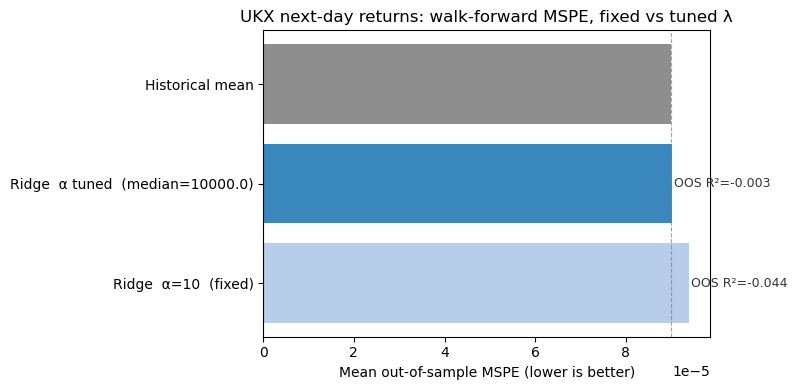
We use **UKX** (FTSE 100 price index) as the target for next-day returns and a small, pre-specified predictor set: the **IVIUK** implied volatility index (the FTSE 100 Implied Volatility Index, the UK counterpart of the VIX) and UK generic gilt yields **GUKG10** and **GUKG2**, each entering through three lags of their daily returns. IVIUK carries a strong negative contemporaneous correlation with UKX returns (-0.67 in the full sample), making it the richest single predictor here. If IVIUK is absent from a parquet built from US-only data, the code falls back to whatever UK risk-gauge series are present.
The block also demonstrates a key practical lesson: **choosing $\lambda$ via nested walk-forward cross-validation** rather than fixing it arbitrarily. Inside each outer training window, a `TimeSeriesSplit` inner loop evaluates a log-grid of penalty values and selects the $\lambda$ that minimises in-window validation MSPE. This is the correct procedure in practice: it respects time ordering at both the inner and outer level and avoids the over-optimism of random K-fold CV. Comparing fixed-$\lambda$ and tuned-$\lambda$ Ridge on the same data shows whether the choice of penalty matters, and what a realistic tuned result looks like on genuinely low signal-to-noise daily returns.
This is a **methods illustration**, not a claim about tradable predictability. Out-of-sample MSPE often lies above the historical-mean benchmark at daily horizons; that is the expected outcome given a low signal-to-noise ratio and does not contradict the role of regularisation in higher-dimensional or lower-frequency settings.
The Bloomberg extract and conversion workflow for building this database are documented in `data/bloomberg_database/UK_BLOOMBERG_EXCEL_DATAWIZARD_CH06.md`. If your local `bloomberg_database.parquet` does not yet contain UKX, the code prints a short notice and skips the figure so the chapter still renders.
```{python}
#| label: fig-uk-bloomberg-walk-forward
#| eval: true
#| fig-cap: "Walk-forward out-of-sample MSPE for next-day UKX returns: fixed-penalty Ridge, nested-CV-tuned Ridge, and historical mean baseline. IVIUK, GUKG10, and GUKG2 (up to 3 lags each) as predictors. Daily data from bloomberg_database.parquet."
#| code-summary: "Show UK Bloomberg walk-forward code"
import numpy as np
import pandas as pd
import matplotlib.pyplot as plt
from sklearn.linear_model import Ridge, RidgeCV
from sklearn.preprocessing import StandardScaler
from sklearn.metrics import mean_squared_error
from sklearn.model_selection import TimeSeriesSplit

TARGET_CANDIDATES = ("UKX", "UKX Index")
# IVIUK = FTSE 100 Implied Volatility Index (UK VIX equivalent); fall back to VFTSE if absent
PREDICTOR_CANDIDATES = ("IVIUK", "VFTSE", "GUKG10", "GUKG2")
LAG_ORDER = (1, 2, 3)
N_INITIAL = 1260          # ~5 years initial training window
N_TEST = 63               # ~1 quarter per test window
ALPHA_FIXED = 10.0        # foil: arbitrary fixed penalty
ALPHA_GRID = np.logspace(-3, 4, 50)   # grid for nested-CV tuning
INNER_CV = TimeSeriesSplit(n_splits=5) # inner walk-forward folds

try:
    bbg = load_bloomberg()
except (FileNotFoundError, Exception) as exc:
    print("UK Bloomberg illustration skipped:", exc)
    bbg = None

if bbg is not None:
    bbg["date"] = pd.to_datetime(bbg["date"])
    avail = set(bbg["ticker"].astype(str).unique())
    target_t = next((c for c in TARGET_CANDIDATES if c in avail), None)
    preds = [p for p in PREDICTOR_CANDIDATES if p in avail]

    if target_t is None:
        print(
            "UK Bloomberg illustration skipped: no UKX series in parquet "
            "(expected ticker UKX or UKX Index after organising a UK Data Wizard export).",
        )
    elif len(preds) == 0:
        print(
            "UK Bloomberg illustration skipped: none of IVIUK, VFTSE, GUKG10, GUKG2 "
            "found in parquet; add a UK risk_gauges export and re-run the organiser.",
        )
    else:
        cols = {}
        for name in [target_t] + preds:
            d = (
                bbg.loc[bbg["ticker"].astype(str) == name, ["date", "return"]]
                .drop_duplicates(subset=["date"])
                .sort_values("date")
            )
            cols[name] = d.set_index("date")["return"]

        panel = pd.DataFrame(cols).dropna(how="any").sort_index()

        # Target: next-day UKX return (shift target back by 1, no lookahead)
        y = panel[target_t].shift(-1)
        X = pd.DataFrame(index=panel.index)
        for p in preds:
            for lag in LAG_ORDER:
                X[f"{p}_L{lag}"] = panel[p].shift(lag)

        valid = X.join(y.rename("y")).dropna()
        valid = valid.replace([np.inf, -np.inf], np.nan).dropna()
        X_df = valid.drop(columns=["y"])
        y_s = valid["y"]
        n = len(valid)

        if n < N_INITIAL + N_TEST + 5:
            print(
                "UK Bloomberg illustration skipped: insufficient aligned rows "
                f"({n}); need a longer UK sample.",
            )
        else:
            fixed_mse, tuned_mse, base_mse = [], [], []
            alphas_chosen = []
            n_windows = (n - N_INITIAL) // N_TEST

            for w in range(n_windows):
                train_end = N_INITIAL + w * N_TEST
                test_end = min(train_end + N_TEST, n)

                X_train = X_df.iloc[:train_end]
                y_train = y_s.iloc[:train_end]
                X_test = X_df.iloc[train_end:test_end]
                y_test = y_s.iloc[train_end:test_end]

                if len(X_test) == 0:
                    continue

                # Scale using training-window statistics only
                scaler = StandardScaler()
                X_tr_sc = scaler.fit_transform(X_train)
                X_te_sc = scaler.transform(X_test)

                # Baseline: training-window historical mean
                mu = float(y_train.mean())
                base_mse.append(mean_squared_error(y_test, np.full(len(y_test), mu)))

                # Model 1: fixed-penalty Ridge (foil — arbitrary choice)
                fixed_mse.append(
                    mean_squared_error(
                        y_test,
                        Ridge(alpha=ALPHA_FIXED).fit(X_tr_sc, y_train).predict(X_te_sc),
                    )
                )

                # Model 2: tuned Ridge — inner TimeSeriesSplit selects lambda
                # Scaler already fitted on training window; inner CV sees scaled data.
                # This is the correct approach: no future data enters at any level.
                rcv = RidgeCV(alphas=ALPHA_GRID, cv=INNER_CV)
                rcv.fit(X_tr_sc, y_train)
                tuned_mse.append(mean_squared_error(y_test, rcv.predict(X_te_sc)))
                alphas_chosen.append(rcv.alpha_)

            if not fixed_mse:
                print(
                    "UK Bloomberg illustration skipped: no completed windows "
                    "(check for non-finite returns after alignment).",
                )
            else:
                mf = float(np.mean(fixed_mse))
                mt = float(np.mean(tuned_mse))
                mb = float(np.mean(base_mse))
                median_alpha = float(np.median(alphas_chosen))

                print(
                    f"Walk-forward result ({len(fixed_mse)} windows, "
                    f"predictors: {preds}, {len(X_df.columns)} features):"
                )
                print(f"  Fixed Ridge  (α={ALPHA_FIXED:.0f}):             "
                      f"MSPE={mf:.4e}   OOS R²={1 - mf/mb:.4f}")
                print(f"  Tuned Ridge  (median α={median_alpha:.2f}):  "
                      f"MSPE={mt:.4e}   OOS R²={1 - mt/mb:.4f}")
                print(f"  Historical mean:                 MSPE={mb:.4e}")

                fig, ax = plt.subplots(figsize=(8, 4))
                labels = [
                    f"Ridge  α={ALPHA_FIXED:.0f}  (fixed)",
                    f"Ridge  α tuned  (median={median_alpha:.1f})",
                    "Historical mean",
                ]
                means = [mf, mt, mb]
                colours = ["#aec7e8", "#1f77b4", "#7f7f7f"]
                bars = ax.barh(labels, means, color=colours, alpha=0.88)
                # Annotate OOS R²
                for bar, mspe in zip(bars[:2], [mf, mt]):
                    r2 = 1 - mspe / mb
                    ax.text(
                        bar.get_width() * 1.005,
                        bar.get_y() + bar.get_height() / 2,
                        f"OOS R²={r2:.3f}",
                        va="center",
                        fontsize=9,
                        color="#333333",
                    )
                ax.set_xlabel("Mean out-of-sample MSPE (lower is better)")
                ax.set_title(
                    "UKX next-day returns: walk-forward MSPE, fixed vs tuned λ",
                    fontsize=12,
                )
                ax.axvline(mb, color="#7f7f7f", linestyle="--", linewidth=0.8, alpha=0.7)
                plt.tight_layout()
                plt.show()
```
The controlled simulation earlier used a fixed $\lambda$ as a simplification. The Bloomberg block now shows what happens with **both** approaches on real data: a fixed $\lambda = 10$ as a foil, and a tuned $\lambda$ selected by an inner `TimeSeriesSplit` walk-forward loop across a log-grid of 50 candidates. The key insight is that the selection procedure itself must respect time ordering: the inner CV uses only training-window data, and the outer evaluation uses only future test data. There is no random shuffling at any stage. The OOS $R^2$ annotations on the chart make the benchmark comparison explicit; for daily index returns, negative values are the expected and honest result [@goyal2008comprehensive], and the gap between fixed and tuned $\lambda$ shows whether the choice of penalty is material in this setting.
## Interpreting Out-of-Sample $R^2$
A useful summary statistic for forecasting performance is the out-of-sample $R^2$, defined as:
$$
R^2_{OOS} = 1 - \frac{\sum_t (r_{t+1} - \hat{r}_{t+1})^2}{\sum_t (r_{t+1} - \bar{r}_t)^2}
$$
where $\hat{r}_{t+1}$ is the model forecast and $\bar{r}_t$ is the expanding-window historical mean. A positive $R^2_{OOS}$ means the model outperforms the historical mean; a negative value means it is worse. @campbell2008predicting show that even small positive values of $R^2_{OOS}$ can translate into meaningful portfolio performance improvements, because the predictor is applied through time. In cross-sectional settings, @gu2020ml show that properly regularised machine learning methods can deliver economically meaningful out-of-sample gains over linear benchmarks, though the magnitude depends on the sample, the feature set, and the evaluation design.
# Part VII: Connections and Extensions {#sec-extensions}
## The Factor Zoo and the Replication Crisis
The theoretical and practical developments in this chapter have significant implications for the current state of the empirical asset pricing literature. @harvey2020false estimate that the t-statistic threshold required to declare a new factor significant, accounting for the number of tests effectively conducted across the literature, should be at least 3.0 rather than the conventional 1.96. Most published factors do not clear this bar.
@jensen2024replication provide a large-scale empirical test of whether the 153 factors in their database survive out-of-sample. They find that many do replicate, but the performance is substantially attenuated relative to the original papers. The attenuation reflects a combination of genuine decay (as arbitrageurs exploit the anomaly) and statistical overfitting in the original research. The machine learning methods in this chapter are both part of the problem (they can mine signals more aggressively than manual research) and part of the solution (proper regularisation and out-of-sample evaluation discipline the search).
## Towards Neural Networks
Random forests and gradient boosting are powerful but still operate on hand-constructed features. The researcher must decide which lags of momentum to include, whether to transform variables, and how to handle missing data. Neural networks take a different approach: they learn feature representations from raw data, potentially discovering transformations that a human analyst would not have considered.
@chen2021deeplearning extend the framework of @gu2020ml to deep networks, finding additional predictive gains in the equity premium and cross-section. The theoretical understanding of why deep networks work in financial prediction is less developed than for the methods covered in this chapter, but the double descent insight applies here too: very large networks trained with appropriate regularisation can outperform smaller networks, even on limited financial datasets. This connects to the broader literature on overparameterised learning surveyed in @belkin2019reconciling.
Chapter 10 of these notes takes up neural networks and their specific challenges in financial applications: time structure, non-stationarity, and the scarcity of labelled data relative to the model capacity deployed. The statistical foundations developed here carry forward directly.
## A Note on Causal Inference
The methods in this chapter are optimised for prediction, not causal identification. A regularised linear model or random forest that achieves positive $R^2_{OOS}$ tells us that some linear combination of the features is associated with future returns in the out-of-sample period. It does not tell us why, whether the association reflects a risk premium or a mispricing, or whether it will persist.
These distinctions matter for portfolio construction and investment strategy. An investor who believes the signal reflects genuine risk would maintain exposure across market conditions; one who believes it reflects mispricing would trade more aggressively and expect decay as arbitrage capital flows in. Machine learning methods as developed here are agnostic about this distinction. Combining them with the causal reasoning of structural asset pricing models, a programme @kellyxiu2023fml describe as "financial machine learning," is an active research frontier.
# Summary
The movement from OLS to machine learning in financial economics is not a fashion shift. It reflects genuine statistical challenges: many predictors, limited observations, strong multicollinearity, and non-linear relationships, challenges that OLS was not designed to handle. The theoretical framework developed in this chapter provides a principled account of when regularisation helps, how to choose among shrinkage methods, and why non-linear methods can outperform linear ones without simply overfitting.
Several themes recur across the methods. The in-sample/out-of-sample distinction is the fundamental one: a method that looks impressive in-sample but fails out-of-sample is worse than useless, because it misleads. Walk-forward validation is the discipline that enforces this distinction in financial settings. The bias-variance tradeoff is the organising framework: each method, from Ridge to random forests, makes a specific trade between these two sources of prediction error, and understanding which trade is appropriate for a given dataset requires thinking carefully about the signal-to-noise ratio and the dimensionality of the problem.
Finally, complexity does not automatically mean better predictions. The double descent result of @kelly2024complexity provides theoretical conditions under which overparameterised models can help, but those conditions include appropriate regularisation and sufficient overparameterisation. Between the interpolation boundary and the genuine overparameterised regime, performance is at its worst. Understanding where any given financial prediction problem sits in this landscape is essential background for any serious application of machine learning to return forecasting.