---
title: "Lab 6: Alternative Finance & Credit Risk Scoring: UCI German Credit"
subtitle: "Real-world credit scoring: UCI German Credit dataset"
format:
html:
toc: true
toc-depth: 2
number-sections: false
execute:
echo: true
eval: true
warning: false
message: false
bibliography:
- ../resources/reading.bib
---
::: {.callout-note}
**Time:** ≈ 60 min core · +20 min extensions
Sample answers are hidden, attempt each question before opening.
[](https://colab.research.google.com/github/quinfer/fin510-colab-notebooks/blob/main/labs/lab06_alt_finance.ipynb)
:::
---
## 0. Setup & Data
We use the [UCI Statlog German Credit dataset](https://archive.ics.uci.edu/dataset/144/statlog+german+credit+data), 1,000 real loan applications from a German bank, 20 features, binary outcome (0 = repaid, 1 = defaulted). This is the same data structure a marketplace lending platform uses to build a scoring model.
```{python}
import pandas as pd
import numpy as np
import matplotlib.pyplot as plt
import warnings
import os
warnings.filterwarnings('ignore')

from sklearn.linear_model import LogisticRegression
from sklearn.model_selection import train_test_split, StratifiedKFold, cross_val_score
from sklearn.preprocessing import StandardScaler
from sklearn.metrics import roc_auc_score, roc_curve
from sklearn.calibration import calibration_curve

# Load German Credit data (works locally and in Colab).
# Try multiple local paths first (Quarto may run from project root or labs/).
# Fall back to UCI source if no local file is found.
_CANDIDATE_PATHS = [
    "../data/alt_finance/german_credit.csv",   # from labs/ directory
    "data/alt_finance/german_credit.csv",       # from project root
    "german_credit.csv",                        # if downloaded in Colab
]
_PUBLIC_MIRROR_URLS = [
    "https://raw.githubusercontent.com/quinfer/fin510-colab-notebooks/main/labs/german_credit.csv",
]
_UCI_URL = (
    "https://archive.ics.uci.edu/ml/machine-learning-databases"
    "/statlog/german/german.data"
)
_UCI_COLS = [
    "checking_status", "duration", "credit_history", "purpose", "credit_amount",
    "savings_status", "employment", "installment_rate", "personal_status",
    "other_parties", "residence_since", "property_magnitude", "age", "other_plans",
    "housing", "existing_credits", "job", "num_dependents", "own_telephone",
    "foreign_worker", "target"
]

df = None
for _path in _CANDIDATE_PATHS:
    if os.path.exists(_path):
        df = pd.read_csv(_path)
        DATA_SOURCE = f"local file ({_path})"
        break

_IS_COLAB = ('COLAB_GPU' in os.environ or 'COLAB_BACKEND_VERSION' in os.environ)
if df is None and _IS_COLAB:
    for _url in _PUBLIC_MIRROR_URLS:
        try:
            df = pd.read_csv(_url)
            DATA_SOURCE = f"public mirror ({_url})"
            break
        except Exception:
            df = None

if df is None:
    _raw = pd.read_csv(_UCI_URL, sep=" ", header=None, names=_UCI_COLS)
    _raw["defaulted"] = (_raw["target"] == 2).astype(int)
    df = _raw.drop(columns="target")
    DATA_SOURCE = "UCI archive (downloaded)"

print(f"Source : {DATA_SOURCE}")
print(f"Shape  : {df.shape[0]} loans × {df.shape[1]} columns")
print(f"Default rate: {df['defaulted'].mean():.1%}  ({df['defaulted'].sum()} defaults)")
```
---
## 1. Explore the Data
> **Before modelling, understand what you're working with.**
```{python}
# Numeric features available
num_cols = [c for c in ['duration', 'credit_amount', 'installment_rate',
                         'age', 'existing_credits', 'num_dependents']
            if c in df.columns]
print(df[num_cols + ['defaulted']].describe().round(1))
```
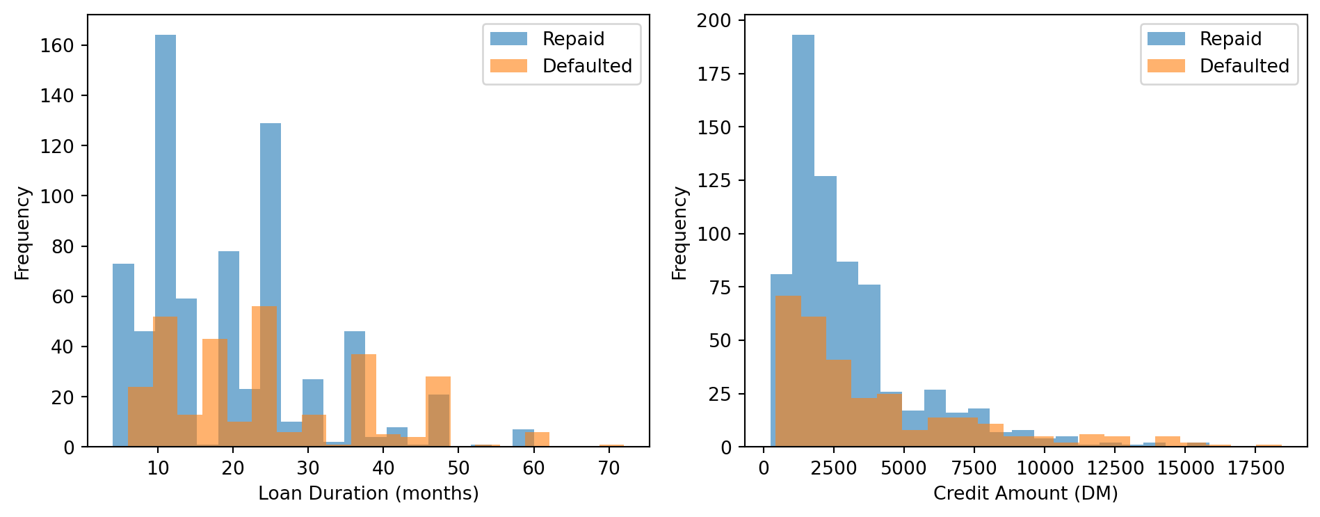
```{python}
# Do defaults vary with duration and credit amount?
if 'duration' in df.columns and 'credit_amount' in df.columns:
    fig, axes = plt.subplots(1, 2, figsize=(10, 4))
    for ax, col, label in zip(axes,
                               ['duration', 'credit_amount'],
                               ['Loan Duration (months)', 'Credit Amount (DM)']):
        for grp, lbl in [(0, 'Repaid'), (1, 'Defaulted')]:
            df.loc[df['defaulted'] == grp, col].plot.hist(
                bins=20, alpha=0.6, ax=ax, label=lbl)
        ax.set_xlabel(label)
        ax.legend()
    plt.tight_layout(); plt.show()
```
> **Q1 (think):** Longer loans appear riskier. Is this a causal relationship, or might duration be a proxy for something else?
::: {.callout-tip collapse="true"}
### Sample Answer
Longer-duration loans have higher default rates for several reasons. First, a longer repayment window increases exposure to life shocks (job loss, illness). Second, larger credit amounts are often granted as longer-term loans, so duration may proxy for amount. Third, lenders sometimes offer longer terms as a concession to higher-risk borrowers, adverse selection embedded in the product design.
Crucially, this is correlation, not causation. Shortening all loans would not automatically reduce defaults. The prediction-vs-causation distinction from Week 1 applies directly: using duration in a predictive model is legitimate, but it does not imply a policy prescription.
:::
---
## 2. Prepare Features
```{python}
# Identify numeric and categorical columns
cat_cols = [c for c in df.columns if df[c].dtype == 'object']

print(f"Numeric  ({len(num_cols)}): {num_cols}")
print(f"Categorical ({len(cat_cols)}): {cat_cols}")
```
```{python}
# Scale numerics; one-hot encode categoricals
scaler = StandardScaler()
X_num = pd.DataFrame(scaler.fit_transform(df[num_cols]), columns=num_cols)

if cat_cols:
    X_cat = pd.get_dummies(df[cat_cols], drop_first=True)
    X_all = pd.concat([X_num, X_cat], axis=1)
else:
    X_all = X_num

y = df['defaulted']
print(f"Feature matrix: {X_all.shape[0]} rows × {X_all.shape[1]} columns")
print(f"  Numeric: {len(num_cols)}  |  One-hot encoded: {X_all.shape[1] - len(num_cols)}")
```
> **Q2 (think):** Why can't we feed the string "A11" directly into logistic regression? What's wrong with converting A11→1, A12→2, A13→3?
::: {.callout-tip collapse="true"}
### Sample Answer
Logistic regression requires numeric inputs with meaningful magnitudes. The string "A11" cannot be interpreted mathematically.
Integer label encoding (A11=1, A12=2, A13=3) implies an ordering that does not exist. The model would infer that category 3 is "three times as large" as category 1, which is meaningless for nominal categories like account type. One-hot encoding creates a separate 0/1 column for each category, allowing the model to learn an independent coefficient per level without imposing any artificial ordering. `drop_first=True` removes one column per feature to avoid perfect multicollinearity (the dummy variable trap).
:::
---
## 3. Baseline: Numeric Features Only
Start simple, fit a model on numeric features alone. This is what a traditional bank might do without credit history records.
```{python}
X_tr, X_te, y_tr, y_te = train_test_split(
    X_num, y, test_size=0.3, random_state=42, stratify=y)

model_num = LogisticRegression(max_iter=1000, random_state=42)
model_num.fit(X_tr, y_tr)

proba_num = model_num.predict_proba(X_te)[:, 1]
auc_num = roc_auc_score(y_te, proba_num)

print(f"Numeric-only AUC: {auc_num:.3f}")
print(f"Baseline (random classifier): 0.500")
```
> **Q3 (think):** AUC ≈ {auc_num:.2f}. In plain English, what does this tell you about the model? Is it good enough for a real lender?
::: {.callout-tip collapse="true"}
### Sample Answer
An AUC of ~0.60–0.70 means the model correctly ranks a random defaulter above a random non-defaulter roughly 60–70% of the time. It is clearly better than random (0.50), but well below what a production credit model needs. Commercial bureau-based models typically achieve 0.75–0.85 using rich payment history. Our numeric-only model uses just six features, with no credit history, savings balance, or employment status, so the gap is expected. It is a useful starting point, not a deployable product.
:::
---
## 4. Richer Model: Add Categorical Features
Now add the coded categorical variables (checking account status, credit history, savings, employment, purpose, etc.) and measure the AUC improvement.
```{python}
X_tr_all, X_te_all, y_tr_all, y_te_all = train_test_split(
    X_all, y, test_size=0.3, random_state=42, stratify=y)

model_all = LogisticRegression(max_iter=2000, random_state=42, C=0.3)
model_all.fit(X_tr_all, y_tr_all)

proba_all = model_all.predict_proba(X_te_all)[:, 1]
auc_all = roc_auc_score(y_te_all, proba_all)

print(f"Numeric-only AUC : {auc_num:.3f}")
print(f"All features AUC : {auc_all:.3f}  (+{auc_all - auc_num:.3f})")
```
```{python}
# Which features push predicted risk up or down most?
coefs = pd.Series(model_all.coef_[0], index=X_all.columns)
print("Top 5: INCREASE default risk")
print(coefs.nlargest(5).round(3).to_string())
print("\nTop 5: DECREASE default risk")
print(coefs.nsmallest(5).round(3).to_string())
```
> **Q4 (think):** Do the top features make economic sense? Are any potentially unfair under UK equality law?
::: {.callout-tip collapse="true"}
### Sample Answer
Features like `checking_status_A11` (overdrawn account) and poor `credit_history` codes make strong economic sense. They directly signal financial distress. `duration` and `credit_amount` increasing risk is also intuitive: larger, longer loans expose lenders to more uncertainty.
`age` typically carries a negative coefficient (older → lower predicted default), which is actuarially plausible but raises a fairness concern. Under the UK Equality Act 2010, age is a protected characteristic in financial services. Using age is legally permissible if there is an objective justification and the difference is proportionate, but a lender must document this and cannot simply argue \"it predicts well.\" The practical concern is that age may be proxying for wealth and stable employment rather than genuine repayment ability, meaning a young applicant with a stable income and good cash flow might be unfairly penalised.
:::
---
## 5. Proper Validation: Cross-Validation
A single train/test split depends on which 300 loans happened to land in the test set, so results can be optimistic or pessimistic by chance. **5-fold stratified cross-validation** gives a stable estimate with honest uncertainty.
```{python}
cv = StratifiedKFold(n_splits=5, shuffle=True, random_state=42)

scores_num = cross_val_score(
    LogisticRegression(max_iter=1000), X_num, y, cv=cv, scoring='roc_auc')
scores_all = cross_val_score(
    LogisticRegression(max_iter=2000, C=0.3), X_all, y, cv=cv, scoring='roc_auc')

print(f"Numeric-only (5-fold): {scores_num.mean():.3f} ± {scores_num.std():.3f}")
print(f"All features (5-fold): {scores_all.mean():.3f} ± {scores_all.std():.3f}")
print(f"\nFold-by-fold (all features): {scores_all.round(3)}")
```
> **Q5 (think):** Compare the CV mean to your single-split result. Is the improvement from adding categorical features consistent across all five folds, or does it disappear in some?
::: {.callout-tip collapse="true"}
### Sample Answer
The CV mean provides a more reliable estimate because it averages over five independent splits, reducing the influence of lucky or unlucky data partitions. If the single-split AUC was notably higher than the CV mean, the single split was optimistically biased.
The standard deviation across folds (e.g. ±0.02–0.03 is typical) tells you about model stability. If the improvement from adding categorical features holds in four out of five folds, it is a genuine signal. If it varies wildly, positive in some folds, negative in others, it suggests the features are noisy rather than consistently informative. In a real deployment decision, you would want the improvement to be stable and larger than the fold-to-fold standard deviation before incurring the engineering cost of collecting and storing categorical data.
:::
---
## 6. Calibration Check
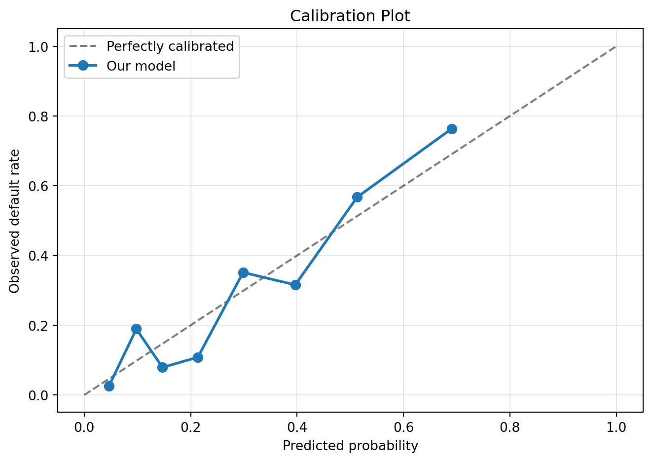
Good AUC means the model ranks risk correctly. **Calibration** checks whether the predicted *numbers* are trustworthy. If the model says "30% default probability", do 30% of those borrowers actually default?
```{python}
prob_true, prob_pred = calibration_curve(y_te_all, proba_all, n_bins=8, strategy='quantile')

fig, ax = plt.subplots(figsize=(7, 5))
ax.plot([0, 1], [0, 1], 'k--', alpha=0.5, label='Perfectly calibrated')
ax.plot(prob_pred, prob_true, 'o-', linewidth=2, markersize=7, label='Our model')
ax.set_xlabel('Predicted probability'); ax.set_ylabel('Observed default rate')
ax.set_title('Calibration Plot'); ax.legend(); ax.grid(alpha=0.3)
plt.tight_layout(); plt.show()

mae = np.mean(np.abs(prob_true - prob_pred))
print(f"Mean calibration error: {mae:.3f}  ({mae*100:.1f} pp on average)")
```
> **Q6 (think):** Is your model over- or under-confident? What goes wrong for a lending platform if the model systematically overestimates default risk?
::: {.callout-tip collapse="true"}
### Sample Answer
A model is overconfident if points lie *above* the diagonal (e.g. predicts 40% default but only 25% actually default). A model is underconfident if points lie *below* (predicts 15% but 30% default).
For a platform, overconfidence means loans are priced too expensively. Borrowers who are genuinely creditworthy are assigned high-risk grades, charged excessive interest rates, or rejected outright. The platform loses market share to competitors who price more accurately, and excludes creditworthy borrowers, exactly the opposite of the inclusion narrative.
Underconfidence is the more dangerous failure: risk is underpriced, investors earn less than expected, capital flees the platform. Calibration is therefore as critical as AUC in production. A model that discriminates perfectly but is 10 percentage points miscalibrated will systematically misjudge loan profitability.
:::
---
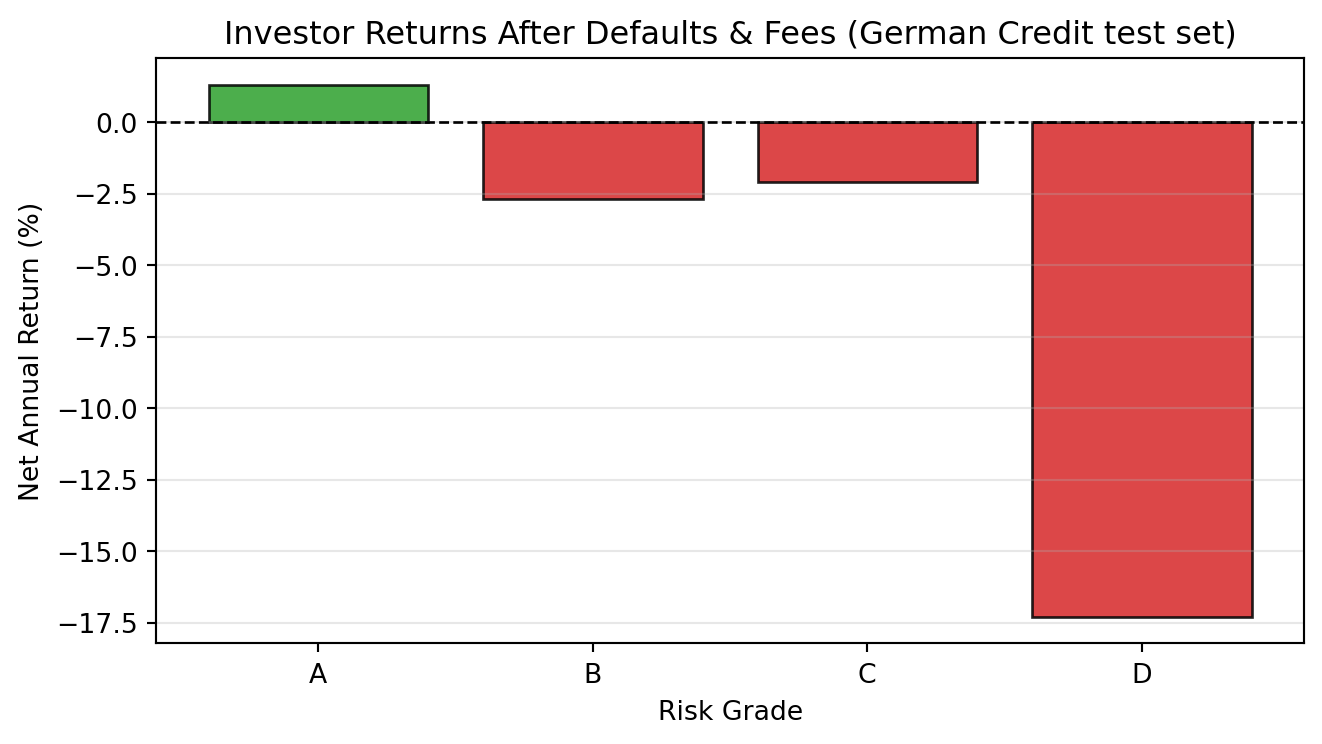
## 7. Risk Grades & Investor Returns
Credit platforms translate predicted probabilities into risk grades (A–D) and set interest rates accordingly. Let's calculate actual investor returns by grade using the German Credit test set.
```{python}
df_te = df.loc[y_te_all.index].copy()
df_te['default_prob'] = proba_all

# Assign grades based on predicted probability
df_te['grade'] = pd.cut(
    df_te['default_prob'],
    bins=[0, 0.20, 0.35, 0.50, 1.01],
    labels=['A', 'B', 'C', 'D'])

# Risk-based interest rates
rate_map = {'A': 0.06, 'B': 0.10, 'C': 0.15, 'D': 0.22}
df_te['rate'] = df_te['grade'].map(rate_map).astype(float)

# Net return: interest minus 1% servicing (if repaid) or annualised principal loss (if defaulted)
df_te['investor_return'] = np.where(
    df_te['defaulted'] == 0,
    df_te['rate'] - 0.01,
    -1.0 / 3)   # lose principal over 3-year loan term

summary = df_te.groupby('grade', observed=True).agg(
    n=('defaulted', 'count'),
    default_rate=('defaulted', 'mean'),
    interest_rate=('rate', 'mean'),
    net_return=('investor_return', 'mean')
).round(3)

print(summary.to_string())
```
```{python}
fig, ax = plt.subplots(figsize=(7, 4))
colors = ['#2ca02c' if r > 0 else '#d62728' for r in summary['net_return']]
ax.bar(summary.index, summary['net_return'] * 100, color=colors, alpha=0.85, edgecolor='k')
ax.axhline(0, color='black', linewidth=1, linestyle='--')
ax.set_xlabel('Risk Grade'); ax.set_ylabel('Net Annual Return (%)')
ax.set_title('Investor Returns After Defaults & Fees (German Credit test set)')
ax.grid(axis='y', alpha=0.3)
plt.tight_layout(); plt.show()
```
> **Q7 (think):** Grade D loans carry 22% interest. Should investors lend to them? What does your result suggest about high-interest lending?
::: {.callout-tip collapse="true"}
### Sample Answer
High interest rates do not guarantee high returns. Grade D loans carry high predicted default probabilities; when a large fraction of borrowers default and investors lose roughly 33% of principal annually on those loans (spread over a 3-year term), the expected net return turns negative even at 22% interest.
This is the \"high-risk trap\" documented in marketplace lending literature: platforms advertise attractive headline rates on risky loans, but actual investor returns depend on whether pricing adequately compensates for realised default losses. Grade A and B loans often deliver better *risk-adjusted* returns because default losses are manageable. A rational investor should focus on expected net return after defaults and fees, not the headline interest rate, precisely the calculation you have just performed. The LendingClub data tells the same story: investors in lower-grade loans often earned less than those in Grade B–C loans, because defaults overwhelmed the extra interest.
:::
---
## 8. Extension: Fairness
The model uses `age`. Older applicants tend to receive better predicted scores.
**Task:** Create an age-group column (e.g. under-30, 30–50, over-50) and compare mean predicted default probability by group. Does the model give systematically better rates to older borrowers?
```{python}
if 'age' in df_te.columns:
    df_te['age_group'] = pd.cut(df_te['age'], bins=[0, 30, 50, 100],
                                  labels=['<30', '30-50', '50+'])
    print(df_te.groupby('age_group', observed=True)[['default_prob', 'defaulted']].mean().round(3))
```
> **Q8 (think):** Is age-based credit scoring fair? When (if ever) is it legally permissible under UK law?
::: {.callout-tip collapse="true"}
### Sample Answer
Under the UK Equality Act 2010, age is a protected characteristic. Using age in a credit model is not automatically unlawful. Section 13 allows for objective justification if the difference in treatment is a proportionate means of achieving a legitimate aim. For a lender, \"predicting default accurately\" is a legitimate aim, and if age genuinely carries independent predictive power beyond other features, its use may be proportionate.
However, the key question is whether age is proxying for wealth, employment stability, or credit history, characteristics that could be measured directly and more fairly. A younger applicant who has stable income, no existing debts, and consistent cash flow may be denied a loan or charged high rates not because of actual risk, but because they have not yet accumulated the credit history that older borrowers carry. This is the inclusion paradox: the very population alternative finance claims to serve (young adults with thin files) is often penalised by the same models meant to include them. Regulators increasingly expect lenders to audit for disparate impact even when the algorithm is facially neutral.
:::