---
title: "Volatility Modelling"
subtitle: "From Stylised Facts to GARCH"
author: "Barry Quinn"
date: last-modified
bibliography: ../resources/reading.bib
format:
html:
toc: true
toc-depth: 3
code-fold: true
execute:
warning: false
message: false
---
## Introduction
Volatility : the tendency of asset prices to fluctuate : is one of the most important concepts in finance. It matters for risk management, option pricing, portfolio construction, and regulatory capital. Yet volatility is not directly observable; we must estimate it from price data.
**Why this chapter matters:** In the [Foundations chapter](01_foundations.qmd), we introduced the Three Prediction Problems in finance: predicting the *mean* (returns), the *variance* (volatility), and *cross-sectional* variation (which assets outperform). We saw that returns have almost no predictable signal (~1-2% R²), making ARIMA largely useless for return prediction. **Volatility is different.** The conditional variance is genuinely predictable (~15-40% R²), and this predictability has direct economic value for options pricing, risk management, and portfolio allocation. This chapter focuses on the second prediction problem: where the signal actually exists.
This chapter develops your understanding of volatility from three perspectives: empirically, by examining what patterns we observe in financial return volatility; theoretically, by showing how ARCH and GARCH models capture these patterns; and practically, by demonstrating how to estimate, forecast, and apply volatility models. By the end of this chapter, you will understand why GARCH(1,1) has become the workhorse model for volatility in finance, and when more sophisticated approaches are needed.
::: {.callout-note}
#### View Slides
Open the lecture deck: [Week 4: Volatility Modelling](../slides/week04_volatility.qmd)
:::
::: {.callout-tip}
## Connection to Week 3
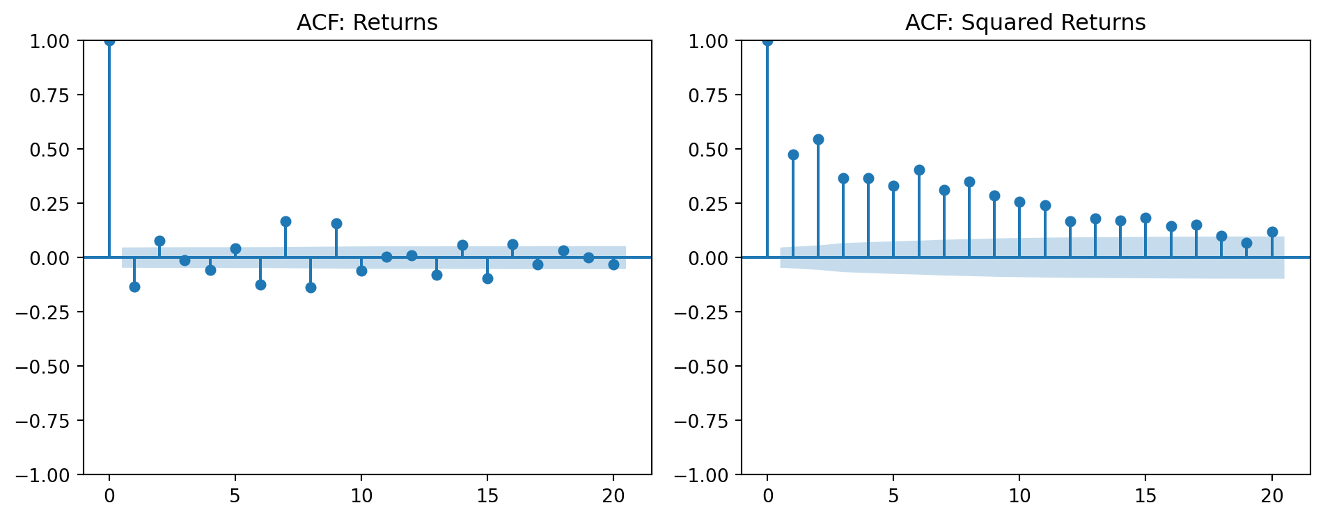
This chapter builds directly on the time series foundations from Week 3. There you learned that the ACF of returns is near zero (no signal in the mean), but the ACF of *squared* returns shows strong persistence. That persistence is volatility clustering: and modelling it is what this chapter is about.
:::
```{python}
#| label: setup-data-root
#| include: false
import sys
from pathlib import Path
sys.path.insert(0, str(Path("scripts").resolve()))
from bloomberg_loader import load_bloomberg
```
## Stylised Facts of Financial Volatility
Before building models, we must understand what we're trying to capture. Financial return volatility exhibits several well-documented patterns : **stylised facts** : that any good model should reproduce.
### Volatility Clustering
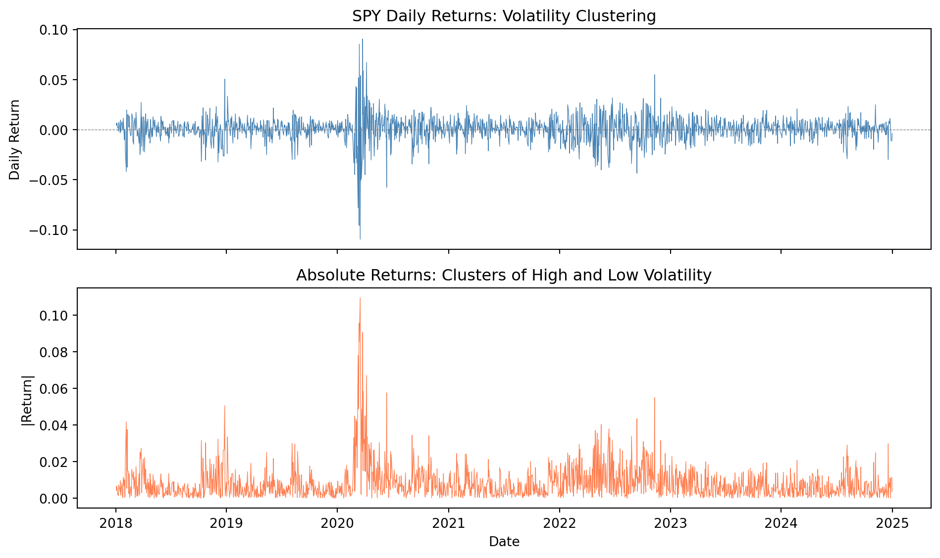
Perhaps the most striking feature of financial returns is **volatility clustering**: large returns (positive or negative) tend to be followed by large returns, and small returns tend to be followed by small returns.
@tsay2010analysis describes this as: "Volatility is not constant over time. There are periods of high volatility alternating with periods of relative calm."
This pattern is visible in virtually every financial time series. The figure below demonstrates clustering in the Bloomberg equity data:
```{python}
#| label: fig-volatility-clustering
#| fig-cap: "Volatility clustering in SPY returns: Large moves cluster together"
import pandas as pd
import numpy as np
import matplotlib.pyplot as plt

# Load Bloomberg database
df = load_bloomberg()

# Get SPY returns
spy = df[df['ticker'] == 'SPY'].set_index('date').sort_index()
returns = spy['PX_LAST'].pct_change().dropna()

# Plot returns
fig, axes = plt.subplots(2, 1, figsize=(10, 6), sharex=True)

# Returns
axes[0].plot(returns.index, returns.values, linewidth=0.5, color='steelblue')
axes[0].axhline(0, color='gray', linestyle='--', linewidth=0.5)
axes[0].set_ylabel('Daily Return')
axes[0].set_title('SPY Daily Returns: Volatility Clustering')

# Absolute returns (proxy for volatility)
axes[1].plot(returns.index, np.abs(returns.values), linewidth=0.5, color='coral')
axes[1].set_ylabel('|Return|')
axes[1].set_xlabel('Date')
axes[1].set_title('Absolute Returns: Clusters of High and Low Volatility')

plt.tight_layout()
plt.show()
```
The autocorrelation structure confirms this pattern: while returns themselves show little autocorrelation (consistent with market efficiency), *squared* returns are highly autocorrelated:
```{python}
#| label: fig-acf-comparison
#| fig-cap: "Returns show no autocorrelation; squared returns do"
from statsmodels.graphics.tsaplots import plot_acf

fig, axes = plt.subplots(1, 2, figsize=(10, 4))

# ACF of returns
plot_acf(returns.dropna(), ax=axes[0], lags=20, title='ACF: Returns')

# ACF of squared returns
plot_acf(returns.dropna()**2, ax=axes[1], lags=20, title='ACF: Squared Returns')

plt.tight_layout()
plt.show()
```
### Fat Tails (Leptokurtosis)
Financial returns consistently exhibit **fatter tails** than the normal distribution predicts. Extreme events : crashes, spikes : occur far more frequently than a Gaussian model would suggest.
@tsay2010analysis notes: "Kurtosis often exceeds three (the kurtosis of a normal distribution), and often exceeds three by a substantial margin."
```{python}
#| label: tbl-distribution-stats
#| tbl-cap: "Financial returns exhibit excess kurtosis"
from scipy import stats

# Calculate statistics for multiple assets
tickers = ['AAPL', 'GOOGL', 'MSFT', 'SPY']
results = []

for ticker in tickers:
    asset = df[df['ticker'] == ticker].set_index('date')['PX_LAST']
    ret = asset.pct_change().dropna()

    results.append({
        'Ticker': ticker,
        'Mean (%)': f"{ret.mean()*100:.3f}",
        'Std (%)': f"{ret.std()*100:.2f}",
        'Skewness': f"{stats.skew(ret):.2f}",
        'Kurtosis': f"{stats.kurtosis(ret):.2f}",
        'Normal?': 'Yes' if stats.kurtosis(ret) < 1 else 'No'
    })

pd.DataFrame(results)
```
### The Leverage Effect
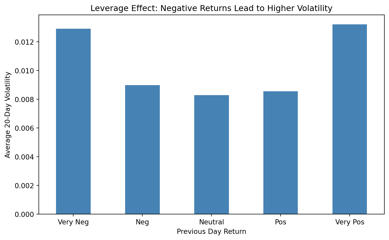
Volatility responds asymmetrically to returns: negative returns tend to increase volatility more than positive returns of the same magnitude. This **leverage effect** was first documented by @black1976studies.
Several theoretical explanations have been proposed:
| Theory | Mechanism | Key Insight |
|--------|-----------|-------------|
| **Leverage hypothesis** | When prices fall, debt/equity ratio rises mechanically | Firms become riskier → volatility increases |
| **Volatility feedback** | If volatility is priced, expected volatility increase raises required return | Causation runs both ways: high volatility → lower prices |
| **Risk premium channel** | Higher expected volatility demands higher risk premium | Current price falls to deliver higher expected return |
| **Behavioural asymmetry** | Investors react more strongly to losses (prospect theory) | Bad news generates more trading, uncertainty |
| **Margin constraints** | Downturns trigger margin calls, forced selling | Amplification through deleveraging cascades |
The leverage hypothesis is the most cited explanation, but @campbell1992no and @bekaert2000asymmetric show that volatility feedback may be equally or more important. In practice, all mechanisms likely operate simultaneously, reinforcing the asymmetric pattern.
```{python}
#| label: fig-leverage-effect
#| fig-cap: "Negative returns increase volatility more than positive returns"
# Calculate rolling volatility and lagged returns
spy_df = df[df['ticker'] == 'SPY'].set_index('date').sort_index()
spy_df['return'] = spy_df['PX_LAST'].pct_change()
spy_df['rolling_vol'] = spy_df['return'].rolling(20).std()
spy_df['lagged_return'] = spy_df['return'].shift(1)

# Bin by lagged return
spy_clean = spy_df.dropna()
spy_clean['return_bin'] = pd.qcut(spy_clean['lagged_return'], q=5, labels=['Very Neg', 'Neg', 'Neutral', 'Pos', 'Very Pos'])

# Plot
fig, ax = plt.subplots(figsize=(8, 5))
spy_clean.groupby('return_bin')['rolling_vol'].mean().plot(kind='bar', ax=ax, color='steelblue')
ax.set_xlabel('Previous Day Return')
ax.set_ylabel('Average 20-Day Volatility')
ax.set_title('Leverage Effect: Negative Returns Lead to Higher Volatility')
ax.tick_params(axis='x', rotation=0)
plt.tight_layout()
plt.show()
```
## The ARCH Model
### Motivation: Conditional Heteroskedasticity
Classical econometrics assumes **homoskedasticity** : constant variance of errors. But volatility clustering tells us this assumption fails for financial data. The variance is not constant; it changes over time in predictable ways.
The key insight of @engle1982autoregressive was to distinguish between **unconditional** and **conditional** variance:
- **Unconditional variance**: The long-run average variance (constant)
- **Conditional variance**: The variance *right now*, given what we know (time-varying)
::: {.callout-important}
## Engle's Key Insight
While the *unconditional* variance of returns may be constant, the *conditional* variance : what we expect given recent information : varies over time in a way we can model.
:::
### The ARCH(q) Specification
The **AutoRegressive Conditional Heteroskedasticity** model specifies:
$$r_t = \mu + \varepsilon_t, \quad \varepsilon_t = \sigma_t z_t, \quad z_t \sim N(0,1)$$
$$\sigma^2_t = \alpha_0 + \alpha_1 \varepsilon^2_{t-1} + \alpha_2 \varepsilon^2_{t-2} + \cdots + \alpha_q \varepsilon^2_{t-q}$$
Where:
- $r_t$ is the return at time $t$
- $\sigma^2_t$ is the **conditional variance** at time $t$
- $\varepsilon^2_{t-1}, \ldots, \varepsilon^2_{t-q}$ are past squared shocks
**Interpretation**: Today's volatility depends on recent *surprises*. If yesterday had a large shock (positive or negative), today's volatility will be elevated.
## The GARCH Model
### From ARCH to GARCH
@bollerslev1986generalized extended ARCH by including lagged conditional variances:
$$\sigma^2_t = \alpha_0 + \alpha_1 \varepsilon^2_{t-1} + \beta_1 \sigma^2_{t-1}$$
This is **GARCH(1,1)** : one ARCH term, one GARCH term. @brooks2019introductory notes:
> "A GARCH(1,1) model will be sufficient to capture the volatility clustering in the data, and rarely is any higher order model estimated or even entertained in the academic finance literature."
### Parameter Interpretation
| Parameter | Name | Interpretation |
|-----------|------|----------------|
| $\alpha_0$ | Constant | Long-run variance floor |
| $\alpha_1$ | ARCH term | Reaction to recent shocks |
| $\beta_1$ | GARCH term | Persistence of volatility |
| $\alpha_1 + \beta_1$ | Persistence | How long shocks affect volatility |
::: {.callout-tip}
## Rule of Thumb
For most financial assets, $\alpha_1 + \beta_1$ is close to (but less than) 1, meaning volatility shocks are highly persistent. Values above 0.9 are typical.
:::
### Why GARCH(1,1) Often Suffices
GARCH(1,1) is remarkably effective for three reasons: parsimony (only 3 parameters capture complex volatility dynamics), memory (the recursive structure implicitly uses the entire history), and mean reversion (volatility eventually returns to its long-run level).
```{python}
#| label: fig-garch-fit
#| fig-cap: "GARCH(1,1) captures volatility dynamics"
#| eval: false
from arch import arch_model

# Fit GARCH(1,1) to SPY
returns_pct = returns * 100  # Scale for numerical stability

model = arch_model(returns_pct.dropna(), vol='Garch', p=1, q=1, mean='Constant')
result = model.fit(disp='off')

# Extract conditional volatility
cond_vol = result.conditional_volatility

# Plot
fig, ax = plt.subplots(figsize=(10, 5))
ax.plot(returns_pct.dropna().index, np.abs(returns_pct.dropna().values),
        alpha=0.3, label='|Returns|', color='steelblue')
ax.plot(cond_vol.index, cond_vol.values,
        label='GARCH(1,1) Conditional Volatility', color='coral', linewidth=1.5)
ax.legend()
ax.set_ylabel('Volatility (%)')
ax.set_title('GARCH(1,1) Fitted Volatility vs Absolute Returns')
plt.tight_layout()
plt.show()

print(result.summary().tables[1])
```
### Stationarity Conditions
For GARCH(1,1) to be **covariance stationary**, we require:
$$\alpha_1 + \beta_1 < 1$$
When this holds, the **unconditional variance** exists:
$$\sigma^2 = \frac{\alpha_0}{1 - \alpha_1 - \beta_1}$$
If $\alpha_1 + \beta_1 = 1$, we have **Integrated GARCH (IGARCH)** : shocks persist forever.
## Asymmetric GARCH Models
Standard GARCH treats positive and negative shocks symmetrically. But the leverage effect suggests this is wrong. Several extensions address this:
### GJR-GARCH
@glosten1993relation add an indicator for negative shocks:
$$\sigma^2_t = \alpha_0 + (\alpha_1 + \gamma I_{t-1}) \varepsilon^2_{t-1} + \beta_1 \sigma^2_{t-1}$$
Where $I_{t-1} = 1$ if $\varepsilon_{t-1} < 0$ (negative shock). The parameter $\gamma$ captures the additional impact of bad news.
### EGARCH
@nelson1991conditional use logarithms to ensure positivity:
$$\ln(\sigma^2_t) = \alpha_0 + \alpha_1 \left( \frac{|\varepsilon_{t-1}|}{\sigma_{t-1}} - \sqrt{2/\pi} \right) + \gamma \frac{\varepsilon_{t-1}}{\sigma_{t-1}} + \beta_1 \ln(\sigma^2_{t-1})$$
The $\gamma$ term directly captures asymmetry.
### Visualising Asymmetry: News Impact Curves
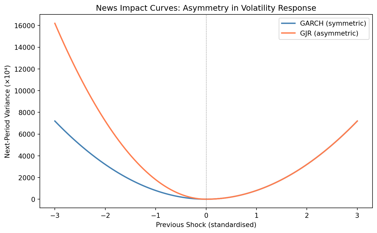
The **news impact curve** (@pagan1990alternative) provides a powerful way to visualise how different shocks affect future volatility. It plots next-period volatility against various values of the previous shock, holding other factors constant.
For a symmetric GARCH model, the curve is a parabola centred at zero : positive and negative shocks of equal magnitude have identical effects. For asymmetric models (GJR, EGARCH), the curve tilts, showing that negative shocks have larger impact.
```{python}
#| label: fig-news-impact
#| fig-cap: "News impact curves: GARCH (symmetric) vs GJR (asymmetric)"
# Simulated news impact curves for illustration
shocks = np.linspace(-3, 3, 100)

# Assume typical parameters
alpha0, alpha1, beta1 = 0.00001, 0.08, 0.90
gamma = 0.10  # Asymmetry parameter for GJR

# GARCH: symmetric response
garch_vol = alpha0 + alpha1 * shocks**2

# GJR: asymmetric - larger response to negative shocks
gjr_vol = alpha0 + (alpha1 + gamma * (shocks < 0)) * shocks**2

fig, ax = plt.subplots(figsize=(8, 5))
ax.plot(shocks, garch_vol * 10000, label='GARCH (symmetric)', color='steelblue', linewidth=2)
ax.plot(shocks, gjr_vol * 10000, label='GJR (asymmetric)', color='coral', linewidth=2)
ax.axvline(0, color='gray', linestyle='--', linewidth=0.5)
ax.set_xlabel('Previous Shock (standardised)')
ax.set_ylabel('Next-Period Variance (×10⁴)')
ax.set_title('News Impact Curves: Asymmetry in Volatility Response')
ax.legend()
plt.tight_layout()
plt.show()
```
The news impact curve reveals that under GJR, a negative shock of magnitude 2 has substantially more impact on future volatility than a positive shock of the same size : consistent with the leverage effect.
## GARCH-M: The Risk-Return Relationship
Standard GARCH models volatility, but doesn't connect it to returns. The **GARCH-in-Mean (GARCH-M)** model (@engle1987estimating) lets volatility enter the mean equation directly:
$$r_t = \mu + \delta \sigma_{t-1} + \varepsilon_t, \quad \varepsilon_t = \sigma_t z_t$$
$$\sigma^2_t = \alpha_0 + \alpha_1 \varepsilon^2_{t-1} + \beta_1 \sigma^2_{t-1}$$
The parameter $\delta$ captures the **risk premium**: if $\delta > 0$, higher expected volatility leads to higher expected returns : compensation for bearing risk.
::: {.callout-note}
## Interpreting GARCH-M
A positive and significant $\delta$ supports the risk-return trade-off from finance theory. However, empirical evidence is mixed : $\delta$ is often insignificant or even negative at short horizons. This may reflect:
- Time-varying risk aversion
- Different risk horizons for different investors
- Measurement error in conditional volatility
:::
## Long Memory in Volatility: IGARCH and Beyond
When $\alpha_1 + \beta_1$ approaches 1, volatility shocks become extremely persistent. The **Integrated GARCH (IGARCH)** model sets $\alpha_1 + \beta_1 = 1$ exactly:
$$\sigma^2_t = \alpha_0 + \beta_1 \sigma^2_{t-1} + (1 - \beta_1) \varepsilon^2_{t-1}$$
@tsay2010analysis notes that under IGARCH, "the impact of past squared shocks... on $\sigma^2_t$ is persistent" : shocks never fully decay. The unconditional variance does not exist.
| Model | Persistence | Unconditional Variance | Use Case |
|-------|-------------|------------------------|----------|
| **GARCH(1,1)** | $\alpha_1 + \beta_1 < 1$ | Exists, finite | Standard applications |
| **IGARCH(1,1)** | $\alpha_1 + \beta_1 = 1$ | Does not exist | Very persistent volatility |
| **FIGARCH** | Fractional integration | Exists | Long memory without unit root |
::: {.callout-warning}
## The IGARCH Puzzle
Finding $\alpha_1 + \beta_1 \approx 1$ is common empirically, but concerning theoretically : it implies volatility shocks persist forever. This may indicate:
- Occasional level shifts in volatility (regime changes)
- Structural breaks misinterpreted as persistence
- Need for a regime-switching specification
:::
## Multivariate Volatility: DCC and Portfolio Applications
When managing portfolios, we need not just individual asset volatilities but **covariances** between assets. Multivariate GARCH models capture time-varying correlations.
### Dynamic Conditional Correlation (DCC)
The **DCC model** (@engle2002dynamic) separates volatility dynamics from correlation dynamics:
$$r_t = \mu_t + D_t z_t$$
Where $D_t$ is a diagonal matrix of univariate GARCH volatilities, and correlations evolve as:
$$Q_t = (1 - \theta_1 - \theta_2)\bar{Q} + \theta_1 \epsilon_{t-1}\epsilon'_{t-1} + \theta_2 Q_{t-1}$$
The correlation matrix is then $R_t = \text{diag}(Q_t)^{-1/2} Q_t \text{diag}(Q_t)^{-1/2}$.
### Application: Time-Varying Hedge Ratios
A key application of multivariate GARCH is computing **optimal hedge ratios** that vary over time. The minimum variance hedge ratio is:
$$h_t = \rho_t \frac{\sigma_{s,t}}{\sigma_{f,t}}$$
Where $\rho_t$ is the conditional correlation between spot and futures returns, and $\sigma_{s,t}, \sigma_{f,t}$ are their conditional volatilities. @brooks2019introductory shows that time-varying hedge ratios from multivariate GARCH often outperform static hedges, particularly during volatile periods.
## Practical Application: VIX and Realised Volatility
### The VIX Index
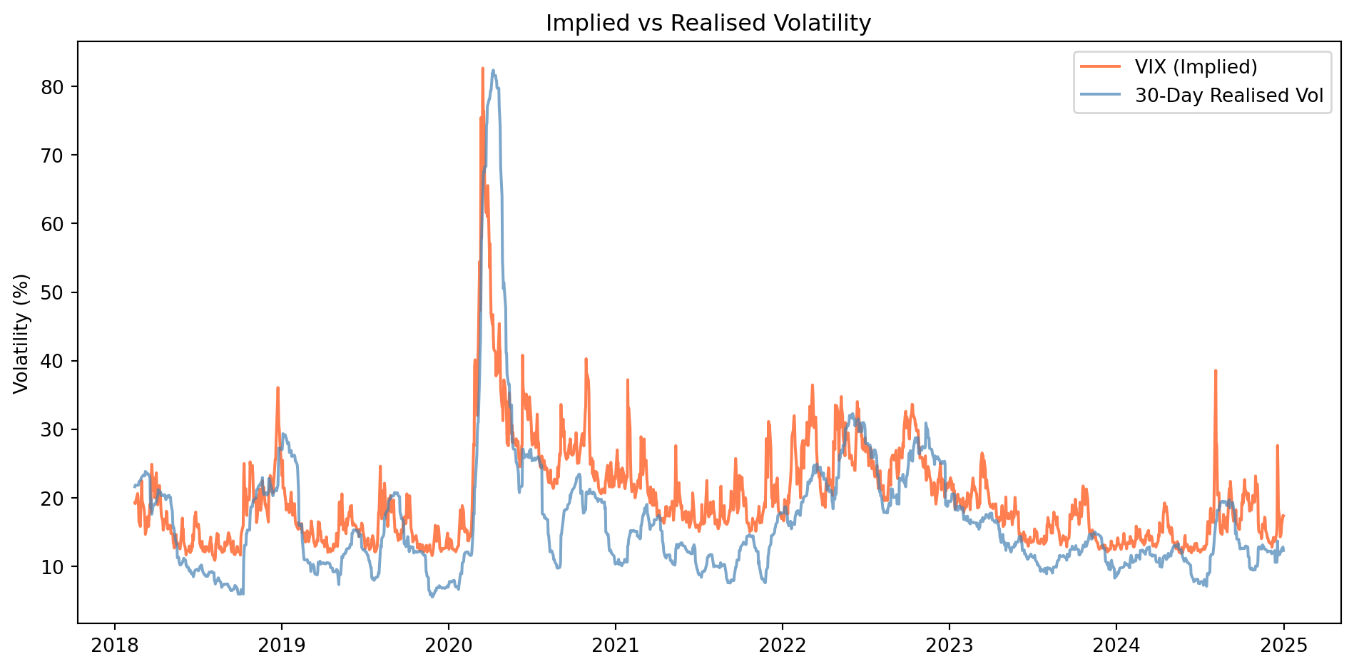
The **VIX** (CBOE Volatility Index) measures the market's expectation of 30-day volatility, extracted from S&P 500 option prices. It represents **implied volatility** : what traders expect.
```{python}
#| label: fig-vix-analysis
#| fig-cap: "VIX (implied) vs SPY realised volatility"
# Load VIX from Bloomberg database
vix = df[df['ticker'] == 'VIX'].set_index('date')['PX_LAST']
spy_close = df[df['ticker'] == 'SPY'].set_index('date')['PX_LAST']

# Calculate 30-day realised volatility (annualised)
spy_ret = spy_close.pct_change()
realised_vol = spy_ret.rolling(30).std() * np.sqrt(252) * 100

# Align dates
common_idx = vix.index.intersection(realised_vol.dropna().index)

fig, ax = plt.subplots(figsize=(10, 5))
ax.plot(common_idx, vix.loc[common_idx], label='VIX (Implied)', color='coral')
ax.plot(common_idx, realised_vol.loc[common_idx], label='30-Day Realised Vol',
        color='steelblue', alpha=0.7)
ax.legend()
ax.set_ylabel('Volatility (%)')
ax.set_title('Implied vs Realised Volatility')
plt.tight_layout()
plt.show()
```
### Volatility Risk Premium
Implied volatility typically exceeds realised volatility : the **volatility risk premium**. This reflects compensation for bearing volatility risk.
## Bayesian Approaches to Volatility
While GARCH models are typically estimated by maximum likelihood, Bayesian methods offer several advantages for volatility modelling : particularly when dealing with parameter uncertainty, model comparison, and complex specifications.
### Why Bayesian Volatility Modelling?
| Challenge | MLE Approach | Bayesian Solution |
|-----------|--------------|-------------------|
| **Parameter uncertainty** | Point estimates + asymptotic SE | Full posterior distributions |
| **Model comparison** | Information criteria (AIC, BIC) | Bayes factors, posterior model probabilities |
| **Small samples** | Unreliable estimates | Priors stabilise inference |
| **Complex models** | Numerical optimisation often fails | MCMC handles high dimensions |
### Stochastic Volatility Models
GARCH treats volatility as a deterministic function of past shocks. **Stochastic volatility (SV)** models treat volatility itself as a random process:
$$r_t = \exp(h_t/2) \varepsilon_t, \quad \varepsilon_t \sim N(0,1)$$
$$h_t = \mu + \phi(h_{t-1} - \mu) + \sigma_\eta \eta_t, \quad \eta_t \sim N(0,1)$$
Where $h_t = \ln(\sigma^2_t)$ is log-volatility, which follows an AR(1) process. The parameter $\phi$ captures volatility persistence; $\sigma_\eta$ captures volatility-of-volatility.
::: {.callout-note}
## SV vs GARCH
- **GARCH**: Volatility is a known function of past data; likelihood is tractable
- **SV**: Volatility is a latent (unobserved) process; requires MCMC or particle filters
SV models often fit financial data better than GARCH (lower in-sample MSE), but GARCH is easier to estimate and produces similar forecasts. The choice depends on whether you need full uncertainty quantification.
:::
### Bayesian GARCH
Even standard GARCH can benefit from Bayesian treatment:
$$\sigma^2_t = \alpha_0 + \alpha_1 \varepsilon^2_{t-1} + \beta_1 \sigma^2_{t-1}$$
With priors:
$$\alpha_0 \sim \text{Gamma}(\cdot), \quad \alpha_1, \beta_1 \sim \text{Beta}(\cdot)$$
The Beta priors on $\alpha_1$ and $\beta_1$ automatically enforce the constraint $0 \leq \alpha_1, \beta_1 \leq 1$. A prior favouring $\alpha_1 + \beta_1$ close to (but less than) 1 incorporates the stylised fact that volatility is highly persistent.
### Practical Benefits
Bayesian approaches to volatility offer three key practical benefits. First, uncertainty propagation: when forecasting volatility, Bayesian methods produce predictive distributions rather than point forecasts, which is essential for risk management since the uncertainty in your volatility estimate should feed into your VaR calculation. Second, shrinkage and regularisation: Bayesian priors prevent extreme parameter estimates that can arise with MLE in small samples, analogous to ridge regression stabilising coefficient estimates. Third, model averaging: rather than selecting a single model, Bayesian model averaging weights predictions from multiple models by their posterior probability, hedging against model misspecification.
::: {.callout-tip}
## The Pragmatic View
For routine volatility forecasting, MLE-GARCH remains the workhorse. Bayesian methods add value when:
- You need full uncertainty quantification for downstream decisions
- You're combining volatility estimates with other uncertain inputs
- You're estimating complex models where MLE struggles
- You want principled model comparison across specifications
:::
## Time-Varying Parameter Models
So far, we've modelled volatility as varying while treating other parameters (mean, coefficients) as constant. But what if the *relationship* between variables changes over time? **State-space models** and the **Kalman filter** provide a general framework for time-varying parameters.
### The State-Space Framework
A state-space model separates what we observe from what we want to estimate:
**Measurement equation** (what we see):
$$y_t = Z_t \alpha_t + \varepsilon_t, \quad \varepsilon_t \sim N(0, H_t)$$
**Transition equation** (how states evolve):
$$\alpha_{t+1} = T_t \alpha_t + R_t \eta_t, \quad \eta_t \sim N(0, Q_t)$$
Where:
- $y_t$ is the observed variable (e.g., returns)
- $\alpha_t$ is the **state vector** (e.g., time-varying beta)
- $Z_t, T_t$ are system matrices defining the model structure
@tsay2010analysis notes: "The Kalman filter is a recursive algorithm for computing the optimal estimator of the state vector at time $t$ based on information available at time $t$."
### Application: Time-Varying Beta (CAPM)
The static CAPM assumes beta is constant:
$$r_{i,t} - r_f = \alpha + \beta (r_{m,t} - r_f) + \varepsilon_t$$
But betas change as firms' risk profiles evolve. A state-space formulation allows beta to drift:
**Measurement:** $r_{i,t} = \alpha_t + \beta_t r_{m,t} + \varepsilon_t$
**State transition:** $\beta_{t+1} = \beta_t + \eta_t$
This is a **random walk** specification for beta : each period's beta equals last period's plus noise. The Kalman filter optimally tracks the evolving beta given the noisy observations.
| Approach | Assumption | Use Case |
|----------|------------|----------|
| **Static regression** | $\beta$ constant forever | Long-run average exposure |
| **Rolling window** | $\beta$ constant within window | Simple adaptation |
| **Kalman filter** | $\beta$ evolves as random walk | Optimal tracking |
| **Regime switching** | $\beta$ jumps between states | Discrete regime changes |
### The Kalman Filter: Predict and Update
The Kalman filter operates in two steps. First, predict: use the transition equation to forecast the state and its uncertainty. Second, update: when new data arrive, combine the forecast with the observation. The **Kalman gain** $K_t$ determines how much weight to give new information versus the forecast : it's automatically higher when the forecast is uncertain or the observation is precise.
::: {.callout-note}
## Connection to Bayesian Inference
The Kalman filter is **Bayesian inference for linear-Gaussian state-space models**:
- The prior is the predicted state distribution
- The likelihood comes from the measurement equation
- The posterior is the updated (filtered) state distribution
For non-linear or non-Gaussian models, extensions like particle filters or MCMC are needed.
:::
### Practical Applications in Finance
| Application | State Variable | What It Captures |
|-------------|----------------|------------------|
| **Time-varying beta** | $\beta_t$ | Evolving systematic risk |
| **Hedging** | Hedge ratio $h_t$ | Changing spot-futures relationship |
| **Factor models** | Factor loadings | Rotating style exposures |
| **Volatility** | $\ln(\sigma^2_t)$ | Stochastic volatility (SV models) |
| **Local trend** | $\mu_t$ | Slowly varying expected return |
### When to Use State-Space Models
State-space models offer several advantages: they handle missing data naturally, provide optimal filtering for signal extraction, quantify uncertainty at each time step, and are flexible enough that many models emerge as special cases. However, they also present challenges: model specification (choosing $T_t$, $Q_t$) requires careful thought, implementation is more complex than GARCH, and computational costs increase substantially for high-dimensional state vectors.
::: {.callout-important}
## The Big Picture
State-space models, regime switching, and GARCH all address the same fundamental problem: financial relationships are not static. They differ in *how* they model non-stationarity:
- **GARCH**: Variance changes, but the *structure* is constant
- **Regime switching**: Parameters jump between discrete states
- **State-space**: Parameters drift continuously
The best choice depends on whether you believe changes are gradual (state-space), abrupt (regime), or only affect volatility (GARCH).
:::
## Structural Breaks and Regime Switching
GARCH models assume that the parameters governing volatility dynamics remain constant over time. But financial markets undergo episodes where behaviour changes dramatically : what @brooks2019introductory calls "very substantial changes in the properties of a series." These changes may be one-off **structural breaks** or recurring **regime switches**.
### What Causes Structural Breaks?
Structural breaks typically result from large-scale events:
| Type | Examples | Effect on Volatility |
|------|----------|---------------------|
| **Policy changes** | Introduction of inflation targeting, QE programmes | May reduce or increase baseline volatility |
| **Market microstructure** | Electronic trading ("Big Bang"), decimal pricing | Often reduces transaction-related volatility |
| **Financial crises** | 2008 GFC, COVID-19 crash | Dramatic volatility regime shift |
| **Regulatory changes** | Basel requirements, Dodd-Frank | May alter risk-taking behaviour |
::: {.callout-important}
## Why Breaks Matter
A linear model (including GARCH) estimated over a sample containing a structural break will be misspecified. The estimated parameters will be a weighted average of the true parameters in each regime : accurate for neither.
:::
### Testing for Structural Breaks
The **Chow test** is the classical approach: split the sample at a suspected break point and test whether the parameters differ significantly between sub-samples. However, this requires *knowing* when the break occurred.
More sophisticated approaches include:
- **CUSUM tests**: Monitor cumulative sums of recursive residuals for evidence of parameter instability
- **Bai-Perron tests**: Detect multiple unknown break points
- **Andrews-Ploberger tests**: Test for breaks at unknown dates
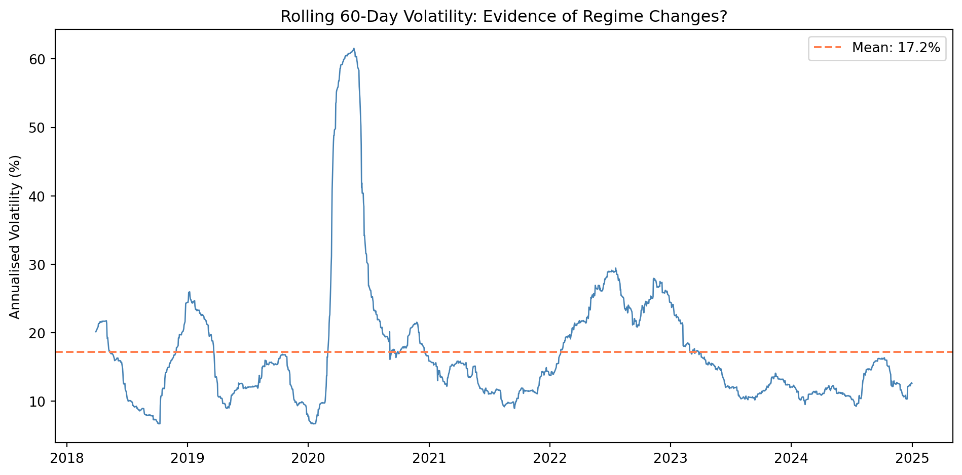
```{python}
#| label: fig-structural-break
#| fig-cap: "Visual inspection for structural breaks in SPY volatility"
# Calculate rolling 60-day volatility
spy_df = df[df['ticker'] == 'SPY'].set_index('date').sort_index()
spy_df['return'] = spy_df['PX_LAST'].pct_change()
spy_df['rolling_vol_60'] = spy_df['return'].rolling(60).std() * np.sqrt(252) * 100

fig, ax = plt.subplots(figsize=(10, 5))
ax.plot(spy_df['rolling_vol_60'].dropna(), color='steelblue', linewidth=1)
ax.axhline(spy_df['rolling_vol_60'].mean(), color='coral', linestyle='--',
           label=f'Mean: {spy_df["rolling_vol_60"].mean():.1f}%')
ax.set_ylabel('Annualised Volatility (%)')
ax.set_title('Rolling 60-Day Volatility: Evidence of Regime Changes?')
ax.legend()
plt.tight_layout()
plt.show()
```
### Markov Switching Models
Rather than treating regime changes as one-off events, **Markov switching models** allow the series to switch between regimes probabilistically. Developed by Hamilton (1989), these models specify that an unobserved **state variable** $z_t$ governs which regime is active.
For a simple two-state model:
$$y_t = \begin{cases}
\mu_1 + \phi_1 y_{t-1} + \sigma_1 u_t & \text{if } z_t = 1 \text{ (calm regime)} \\
\mu_2 + \phi_2 y_{t-1} + \sigma_2 u_t & \text{if } z_t = 2 \text{ (turbulent regime)}
\end{cases}$$
The state evolves according to **transition probabilities**:
$$P = \begin{pmatrix} p_{11} & 1 - p_{11} \\ 1 - p_{22} & p_{22} \end{pmatrix}$$
Where $p_{11}$ is the probability of staying in regime 1 given we were in regime 1, and $p_{22}$ is the probability of staying in regime 2.
::: {.callout-note}
## The Markov Property
A process has the Markov property if the probability of being in a given state depends *only* on the previous state, not on the entire history. This makes estimation tractable while still capturing regime persistence.
:::
### Threshold Autoregressive (TAR) Models
An alternative approach makes regime switches **deterministic** rather than probabilistic. In a **Self-Exciting Threshold AutoRegressive (SETAR)** model, the regime depends on whether a threshold variable exceeds a critical value:
$$y_t = \begin{cases}
\phi^{(1)}_0 + \phi^{(1)}_1 y_{t-1} + \varepsilon_t & \text{if } y_{t-d} \leq c \\
\phi^{(2)}_0 + \phi^{(2)}_1 y_{t-1} + \varepsilon_t & \text{if } y_{t-d} > c
\end{cases}$$
Where $c$ is the **threshold** and $d$ is the **delay parameter**.
| Model Type | Regime Determination | Estimation | Use Case |
|------------|---------------------|------------|----------|
| **Markov Switching** | Probabilistic (latent state) | MLE with Hamilton filter | When switching is random/unpredictable |
| **SETAR** | Deterministic (observable variable) | NLS with grid search | When switching depends on observed values |
### Regime-Switching GARCH
Combining regime switching with GARCH captures both volatility clustering *within* regimes and shifts *between* regimes:
$$\sigma^2_t = \begin{cases}
\alpha_0^{(1)} + \alpha_1^{(1)} \varepsilon^2_{t-1} + \beta_1^{(1)} \sigma^2_{t-1} & \text{if calm regime} \\
\alpha_0^{(2)} + \alpha_1^{(2)} \varepsilon^2_{t-1} + \beta_1^{(2)} \sigma^2_{t-1} & \text{if turbulent regime}
\end{cases}$$
This is particularly useful for modelling financial crises, where not only the *level* of volatility changes but also its *dynamics*.
## From Classical Models to Sequence Learning
The models discussed so far : GARCH, Markov switching, TAR : represent the classical econometric approach to time-varying volatility. Modern machine learning offers powerful extensions through **sequence models** that can capture more complex temporal dependencies.
### The Conceptual Bridge
Consider the parallel between classical and modern approaches:
| Classical Concept | ML Extension | Key Advance |
|-------------------|--------------|-------------|
| **AR(p)** process | Recurrent Neural Network (RNN) | Non-linear dependencies, learned representations |
| **Markov switching** | Hidden Markov Model (HMM) | More flexible state dynamics |
| **GARCH** | LSTM/GRU networks | Long-range memory without explicit structure |
| **Regime detection** | Change point detection | Automated, data-driven identification |
### Recurrent Neural Networks as Non-Linear AR Models
A **recurrent neural network** (RNN) extends the autoregressive framework to allow non-linear dependencies:
$$h_t = f(W_h h_{t-1} + W_x x_t + b)$$
$$y_t = g(W_y h_t + c)$$
Where $h_t$ is a **hidden state** that captures information from the entire history. @dixon2020machine describe RNNs as "non-linear time series models [that] generalise classical linear time series models such as AR(p)."
::: {.callout-tip}
## Why This Matters for Finance
RNNs can learn complex patterns in volatility that GARCH cannot capture:
- Non-linear responses to shocks
- Interactions between multiple assets
- Regime-dependent dynamics (without pre-specifying regimes)
:::
### Long Short-Term Memory (LSTM)
Standard RNNs struggle with **long-range dependencies** : the vanishing gradient problem. **LSTM** networks address this with gated mechanisms that control information flow: a forget gate (what to discard from memory), an input gate (what new information to store), and an output gate (what to reveal to the next layer).
This architecture is particularly relevant for financial time series where volatility shocks can have persistent effects, market regimes may last months or years, and multiple timescales interact (daily noise, weekly patterns, monthly cycles).
### Practical Implications
The connection between classical econometrics and modern ML is not merely theoretical. Consider four key trade-offs. Interpretability versus flexibility: GARCH parameters have direct economic meaning (persistence, reaction to news), whereas neural networks offer flexibility but less transparency. Data requirements: GARCH can be estimated reliably with hundreds of observations, but deep learning typically requires thousands or millions. Out-of-sample performance: simple GARCH often outperforms complex ML models for volatility forecasting : a reminder that more parameters does not equal better predictions. Finally, hybrid approaches that combine GARCH-type structure with neural network flexibility (such as Neural GARCH) may offer the best of both worlds.
::: {.callout-important}
## The Fundamental Challenge
Whether using GARCH or LSTM, the core challenge remains: volatility is **unobservable**. We estimate it from returns, but we never see the "true" volatility to evaluate our models against. This is why comparing implied vs realised volatility, and testing forecasts against future squared returns, remains essential.
:::
## Summary
| Concept | Key Point |
|---------|-----------|
| **Volatility clustering** | Large returns follow large returns |
| **Fat tails** | Extreme events more common than normal |
| **Leverage effect** | Bad news increases volatility more than good news |
| **ARCH** | Conditional variance depends on past shocks |
| **GARCH(1,1)** | Adds persistence; often sufficient |
| **Asymmetric GARCH** | GJR-GARCH, EGARCH capture leverage |
| **News impact curve** | Visualises asymmetric volatility response |
| **GARCH-M** | Volatility in mean equation; risk premium |
| **IGARCH** | Unit-root persistence; unconditional variance undefined |
| **DCC** | Dynamic correlations for multivariate volatility |
| **Stochastic volatility** | Volatility as latent process; requires MCMC |
| **Bayesian GARCH** | Full uncertainty quantification; regularisation |
| **State-space models** | Time-varying parameters via Kalman filter |
| **Time-varying beta** | Evolving systematic risk exposure |
| **Structural breaks** | One-off changes in series behaviour |
| **Markov switching** | Probabilistic regime changes (Hamilton) |
| **TAR/SETAR** | Deterministic threshold-based regimes |
| **Sequence learning** | RNN/LSTM as non-linear AR extensions |
| **VIX** | Market's expectation of future volatility |
::: {.callout-note}
## What's Next?
In the lab, you'll estimate GARCH models on the Bloomberg data, compare implied vs realised volatility, explore whether asymmetric models improve forecasts, and investigate evidence of regime changes.
:::
## References