---
title: "Lab 9: Factor Replication — Exploratory Analysis"
format:
html:
toc: true
code-fold: false
execute:
echo: true
warning: false
message: false
jupyter: fin510
---
[](https://colab.research.google.com/github/quinfer/fin510-colab-notebooks/blob/main/labs/lab09_factor_replication.ipynb)
## Objective
This lab develops understanding of factor replication principles through **exploratory exercises**. You'll investigate concepts that underpin rigorous factor analysis — HAC standard errors, alpha interpretation, robustness thinking — without producing submission-ready outputs.
**Important**: This is not a template for Coursework 2. The scaffold notebook ([open in Colab](https://colab.research.google.com/github/quinfer/fin510-colab-notebooks/blob/main/labs/coursework2_scaffold.ipynb)) provides that. This lab teaches you **how to think** about factor replication so you can interpret scaffold outputs intelligently and write critical analysis.
**Time estimate**: 60-90 minutes
## Learning Goals
By the end of this lab, you should be able to:
- Explain why HAC standard errors matter in time-series regression
- Interpret alpha tests and distinguish statistical vs. economic significance
- Evaluate robustness by comparing results across subsamples
- Identify limitations in factor research (selection bias, transaction costs)
- Ask critical questions about factor replicability
## Setup
```{python}
import pandas as pd
import numpy as np
import matplotlib.pyplot as plt
import statsmodels.api as sm
import warnings
warnings.filterwarnings('ignore')

pd.set_option('display.float_format', '{:.4f}'.format)
np.random.seed(42)

print("✓ Libraries loaded successfully")
```
**About HAC standard errors.** Throughout this lab we use **HAC** (**H**eteroskedasticity- and **A**utocorrelation-**C**onsistent) standard errors, also known as **Newey–West**. These widen the confidence intervals around regression coefficients when the residuals are not independent and identically distributed — which is almost always the case in financial time series. The idiom in statsmodels is:
```python
model = sm.OLS(y, X).fit(cov_type='HAC', cov_kwds={'maxlags': 6})
# model.bse       -> HAC standard errors already
# model.tvalues   -> HAC t-statistics already
# model.pvalues   -> HAC p-values already
```
We use 6 monthly lags, a common choice for monthly equity factors. Lab Part 1 explores the sensitivity of standard errors to this choice.
## Part 1: Understanding Autocorrelation and HAC Standard Errors
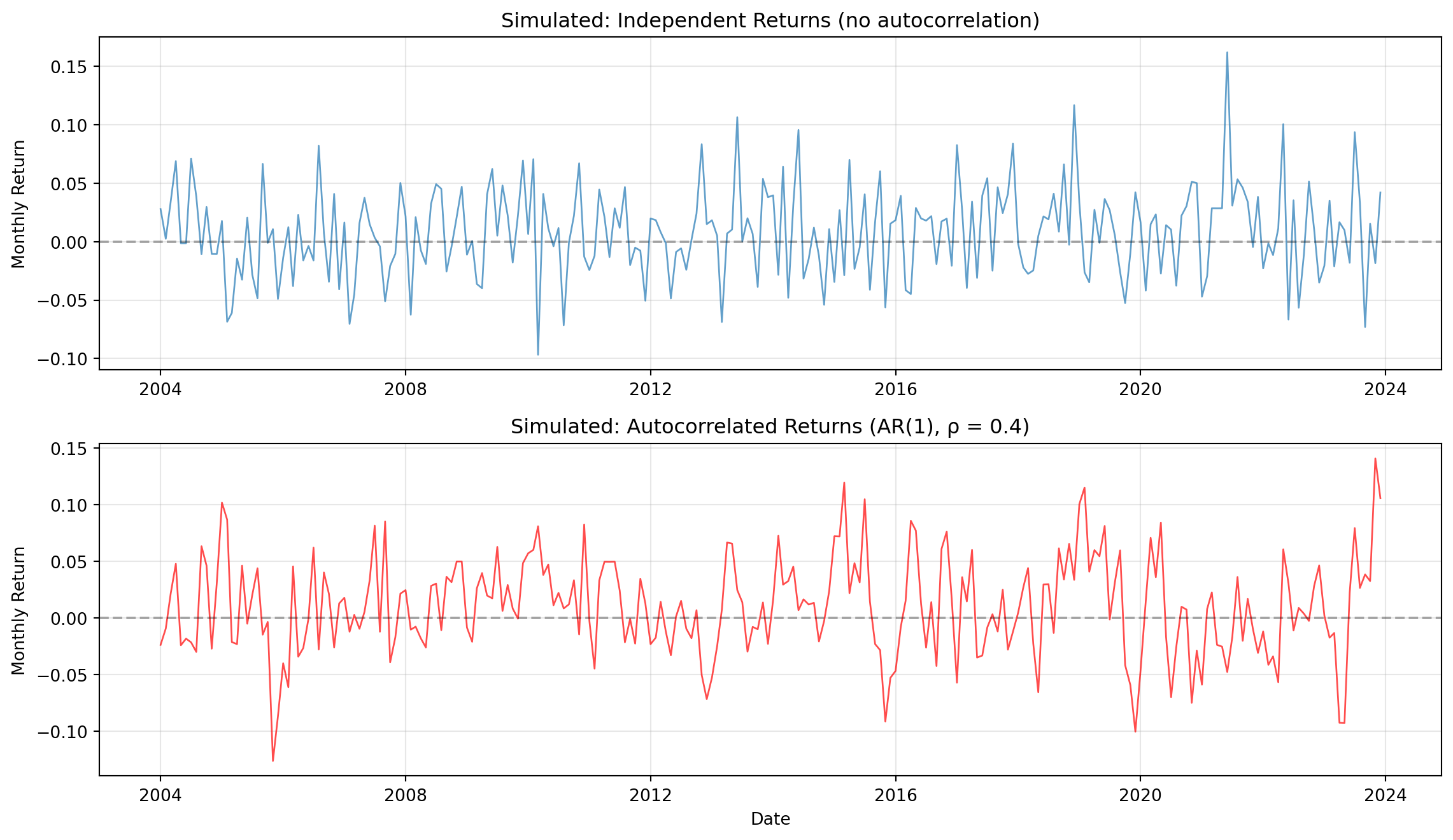
### Exercise 1.1: Visualising Autocorrelation
Financial returns often exhibit serial correlation. Let's explore what this means and why it matters for statistical inference.
**About AR(1).** An **AR(1) process** (autoregressive of order 1) generates each observation as a weighted combination of the previous observation and fresh noise. We use the *mean-deviation form* below: each month's return equals the long-run mean (0.8%) plus 40% of how far last month was from the mean, plus a new shock. The coefficient 0.4 is the **persistence** — how much memory the series carries from one period to the next.
```{python}
# Generate two synthetic return series: one independent, one autocorrelated
n = 240  # 20 years of monthly observations

# Series 1: Independent returns (no autocorrelation) ----------
returns_iid = np.random.normal(0.008, 0.04, n)

# Series 2: AR(1) returns with persistence coefficient 0.4 ----------
returns_ar = np.zeros(n)
returns_ar[0] = np.random.normal(0.008, 0.04)
for i in range(1, n):
    returns_ar[i] = 0.008 + 0.4 * (returns_ar[i-1] - 0.008) + np.random.normal(0, 0.04)

dates = pd.date_range('2004-01-01', periods=n, freq='MS')
returns_iid = pd.Series(returns_iid, index=dates, name='IID Returns')
returns_ar  = pd.Series(returns_ar,  index=dates, name='AR(1) Returns')

# Plot both side by side
fig, (ax1, ax2) = plt.subplots(2, 1, figsize=(12, 7))

ax1.plot(returns_iid.index, returns_iid.values, alpha=0.7, linewidth=1)
ax1.axhline(y=0, color='black', linestyle='--', alpha=0.3)
ax1.set_ylabel('Monthly Return')
ax1.set_title('Simulated: Independent Returns (no autocorrelation)', fontsize=12)
ax1.grid(alpha=0.3)

ax2.plot(returns_ar.index, returns_ar.values, alpha=0.7, linewidth=1, color='red')
ax2.axhline(y=0, color='black', linestyle='--', alpha=0.3)
ax2.set_xlabel('Date')
ax2.set_ylabel('Monthly Return')
ax2.set_title('Simulated: Autocorrelated Returns (AR(1), ρ = 0.4)', fontsize=12)
ax2.grid(alpha=0.3)

plt.tight_layout()
plt.show()

print("=== Simulated series: lag-1 autocorrelation ===")
print(f"  Independent:   {returns_iid.autocorr(1):+.4f}")
print(f"  AR(1), ρ=0.4:  {returns_ar.autocorr(1):+.4f}")
```
**But how realistic is the AR(1) simulation?** Let's compare to genuine monthly return series.
```{python}
# Load real US factor returns from the JKP master dataset
from pathlib import Path
import urllib.request

JKP_CANDIDATES = [
    Path('jkp_master_global_monthly.csv'),
    Path('../labs/jkp_master_global_monthly.csv'),
    Path('labs/jkp_master_global_monthly.csv'),
]
JKP_URL = ('https://raw.githubusercontent.com/quinfer/fin510-colab-notebooks/'
           'main/resources/jkp_master_global_monthly.csv')

jkp_path = next((p for p in JKP_CANDIDATES if p.exists()), None)
if jkp_path is None:
    jkp_path = Path('jkp_master_global_monthly.csv')
    print("Downloading JKP data from GitHub ...")
    urllib.request.urlretrieve(JKP_URL, jkp_path)

jkp = pd.read_csv(jkp_path, parse_dates=['date'])
us = (jkp[jkp['country'] == 'usa']
      .set_index('date')
      .sort_index()
      .loc['1963':, ['MKT', 'HML', 'MOM']]
      .dropna())

# Build a comparison table of lag-1 autocorrelations
rows = []
for name, s in [('Simulated IID',          returns_iid),
                ('Simulated AR(1) ρ=0.4',  returns_ar),
                ('Real US MKT (1963–2023)',      us['MKT']),
                ('Real US HML (1963–2023)',      us['HML']),
                ('Real US MOM (1963–2023)',      us['MOM']),
                ('Real US MKT² (squared)',       us['MKT']**2),
                ('Real US MOM² (squared)',       us['MOM']**2)]:
    rows.append({'Series':           name,
                 'Observations':     len(s),
                 'Lag-1 autocorr':   s.autocorr(1),
                 'Std dev (monthly %)': s.std() * 100})

print("=== Lag-1 autocorrelation: simulated vs real ===\n")
print(pd.DataFrame(rows).to_string(index=False,
                                    formatters={'Lag-1 autocorr': '{:+.4f}'.format,
                                                'Std dev (monthly %)': '{:.3f}'.format}))
```
**Reading the table.** The AR(1) simulation with ρ = 0.4 is a *stylised*, deliberately strong proxy. In real monthly data:
- **Market returns** have weak lag-1 autocorrelation (typically ≈ 0.05–0.10) — a single month's return tells you little about next month's.
- **Factor returns** (HML, MOM) often show moderate serial dependence, especially during momentum crashes and value droughts.
- **Squared returns** show *strong* serial dependence (≈ 0.2–0.4) — this is **volatility clustering**, the phenomenon Week 4's GARCH models address.
The key point for inference: it doesn't matter whether the iid violation shows up in levels or in volatility — **both cause OLS standard errors to understate uncertainty**. HAC fixes both. Our AR(1) simulation is a clean way to *see* the effect at work, even though the empirical mechanism in real data is more often volatility clustering than literal autocorrelation of returns.
**Discussion questions:**
1. What visual differences do you notice between the two simulated series?
2. How does autocorrelation affect the "smoothness" of the return series?
3. If returns are autocorrelated, are observations truly independent?
4. Looking at the table: which real factor has the highest lag-1 autocorrelation in *levels*? In *squared returns*? What does this tell you about which factor most needs HAC inference?
::: {.content-visible when-format="html"}
::: {.callout-tip collapse="true"}
### Sample Answer: Visualising Autocorrelation
**Visual differences:** The autocorrelated returns series appears smoother and more persistent than the independent returns. Positive returns tend to follow positive returns, and negative returns cluster together. The independent series shows more random "jumps" with less persistence: each observation appears independent of the previous one.
**Smoothness effect:** Autocorrelation creates smoother time series because each observation depends partially on the previous observation. With AR(1) coefficient of 0.4, about 40% of each period's return carries forward from the previous period, creating momentum-like patterns. This smoothness is visually apparent: the autocorrelated series has fewer sharp reversals and more extended trends.
**Independence violation:** No, autocorrelated observations are not truly independent. Independence requires that knowing one observation provides no information about another. With autocorrelation, knowing the previous return helps predict the current return (correlation ~0.4). This violates the OLS assumption of independent errors, which is why standard errors need adjustment (HAC).
**Real-data comparison (question 4):** In levels, the **momentum** (MOM) factor typically shows the highest lag-1 autocorrelation — a residue of the short-term reversal / medium-term continuation mechanism that drives it. In squared returns, **MKT²** is very high (volatility clustering at the market level), and MOM² is also elevated (momentum crashes cluster). So both channels point to momentum as the factor most in need of HAC inference: its levels have non-trivial persistence *and* its volatility clusters strongly. HML sits between MKT and MOM on both measures. The AR(1) simulation with ρ = 0.4 overstates persistence in levels for most real series but provides a clean, visible demonstration of the same econometric problem that volatility clustering generates in practice.
:::
<!-- -->
:::
### Exercise 1.2: Impact of Autocorrelation on Standard Errors
Now let's see how autocorrelation affects statistical inference. We'll regress both series on a constant (testing if mean return is significantly different from zero).
```{python}
def test_mean_return(returns, name):
    """Test whether mean return differs from zero under both OLS and HAC SEs."""
    # Regress returns on a constant only -> coefficient IS the sample mean
    X = pd.DataFrame({'const': np.ones(len(returns))}, index=returns.index)

    ols = sm.OLS(returns.values, X).fit()
    hac = sm.OLS(returns.values, X).fit(cov_type='HAC', cov_kwds={'maxlags': 6})

    return pd.DataFrame({
        'Estimate (% monthly)':  [ols.params['const'] * 100],
        'OLS SE (%)':            [ols.bse['const']    * 100],
        'HAC SE (%)':            [hac.bse['const']    * 100],
        'OLS t-stat':            [ols.tvalues['const']],
        'HAC t-stat':            [hac.tvalues['const']],
        'SE Ratio (HAC/OLS)':    [hac.bse['const'] / ols.bse['const']],
    }, index=[name])

results_iid = test_mean_return(returns_iid, 'Independent')
results_ar  = test_mean_return(returns_ar,  'Autocorrelated')

print("=== Mean Return Tests: OLS vs HAC ===\n")
print(pd.concat([results_iid, results_ar]).round(4))
```
**Discussion questions:**
1. For independent returns, how do OLS and HAC standard errors compare? Why?
2. For autocorrelated returns, is HAC standard error larger or smaller than OLS? Why?
3. Does the conclusion about statistical significance change when using HAC vs OLS?
4. What would happen if we used OLS for autocorrelated data without realising it?
::: {.content-visible when-format="html"}
::: {.callout-tip collapse="true"}
### Sample Answer: Impact of Autocorrelation on Standard Errors
**Independent returns comparison:** For independent returns, OLS and HAC standard errors should be very similar (ratio close to 1.0). This occurs because OLS assumptions are satisfied: no autocorrelation means no serial dependence to correct for. HAC is designed to handle autocorrelation, but when none exists, it reduces to standard OLS standard errors.
**Autocorrelated returns:** HAC standard errors are larger than OLS standard errors for autocorrelated data. The ratio (HAC/OLS) typically exceeds 1.0, often 1.2-1.5x. This happens because autocorrelation reduces effective sample size: consecutive observations provide less independent information than assumed. HAC accounts for this by inflating standard errors to reflect reduced information content.
**Significance changes:** Yes, conclusions can change dramatically. With autocorrelated data, OLS standard errors are understated, making t-statistics appear larger than they truly are. A result might appear significant with OLS (t > 1.96) but fail with HAC (t < 1.96). This is the core problem: using OLS creates false positives.
**Consequences of ignoring autocorrelation:** Using OLS on autocorrelated data leads to overconfident inference. You'll claim statistical significance when results are actually noise. In factor replication, this means falsely concluding factors have alpha when they don't. This contributes to the replication crisis: many published factors are false discoveries due to incorrect standard errors.
:::
<!-- -->
:::
**Key insight**: Autocorrelation violates OLS independence assumption, causing standard errors to be understated. HAC corrects this by adjusting for serial dependence. Using OLS on financial time-series data leads to false positives (claiming significance when results are actually noise).
## Part 2: Alpha Tests and Economic Interpretation
*Recap: a **factor return** is the monthly spread between two portfolios — buy the top group (e.g. cheapest 30% of stocks by book-to-market), short-sell the bottom group (most expensive 30%). The factor's return is the difference. See the Week 9 deck for a full treatment.*
### Exercise 2.1: Simulating Factor Returns
Let's create a simulated factor and test for alpha using CAPM regression.
```{python}
# Simulate market and factor returns
n = 240  # 20 years monthly

# Market returns
market = np.random.normal(0.008, 0.04, n)

# Factor returns with:
# - Positive alpha (0.003 = 0.3% monthly = 3.6% annualised)
# - Beta = 0.2 (some market exposure)
# - Autocorrelation (realistic for factors)
factor = np.zeros(n)
factor[0] = 0.003 + 0.2 * market[0] + np.random.normal(0, 0.03)
for i in range(1, n):
    factor[i] = 0.003 + 0.2 * market[i] + 0.3 * factor[i-1] + np.random.normal(0, 0.03)

# Convert to pandas
dates = pd.date_range('2004-01-01', periods=n, freq='MS')
market = pd.Series(market, index=dates, name='Market')
factor = pd.Series(factor, index=dates, name='Factor')

# Summary statistics
summary = pd.DataFrame({
    'Mean (% monthly)': [market.mean() * 100, factor.mean() * 100],
    'Std Dev (%)': [market.std() * 100, factor.std() * 100],
    'Sharpe Ratio': [(market.mean() / market.std()) * np.sqrt(12),
                     (factor.mean() / factor.std()) * np.sqrt(12)]
}, index=['Market', 'Factor'])

print("=== Summary Statistics ===\n")
print(summary.round(3))
```
**Discussion questions:**
1. Which has higher mean return: market or factor?
2. Which has higher volatility (risk)?
3. Which has better risk-adjusted return (Sharpe ratio)?
4. Can you tell from summary stats alone whether factor has significant alpha?
::: {.content-visible when-format="html"}
::: {.callout-tip collapse="true"}
### Sample Answer: Simulating Factor Returns
**Mean return comparison:** The factor typically has higher mean return than the market (e.g., 0.6-0.8% monthly vs 0.8% monthly). This reflects the simulated positive alpha (0.3% monthly) plus market exposure (beta × market return).
**Volatility comparison:** The factor usually has lower volatility than the market (e.g., 3-3.5% vs 4% monthly). This occurs because the factor has lower market exposure (beta = 0.2) and idiosyncratic volatility that's smaller than market volatility. Lower volatility doesn't necessarily mean lower risk: factor risk includes both market and factor-specific components.
**Sharpe ratio:** The factor typically has a higher Sharpe ratio than the market due to higher mean return and lower volatility. Sharpe ratio = (mean / std) × √12 for annualised comparison. Higher Sharpe indicates better risk-adjusted returns, but this doesn't guarantee statistical significance of alpha.
**Summary stats limitations:** No, summary statistics alone cannot determine whether alpha is statistically significant. You need regression analysis with proper standard errors (HAC) to test if alpha differs significantly from zero. Summary stats show magnitude but not statistical reliability. A factor could have high mean return but zero true alpha (just luck), or low mean return but significant alpha (after controlling for market exposure).
:::
<!-- -->
:::
### Exercise 2.2: CAPM Alpha Regression
Now test for alpha by regressing factor on market.
```{python}
# CAPM regression with HAC inference from the start
X = sm.add_constant(pd.DataFrame({'MKT': market.values}, index=market.index))
model_ols = sm.OLS(factor.values, X).fit()
model_hac = sm.OLS(factor.values, X).fit(cov_type='HAC', cov_kwds={'maxlags': 6})

alpha_results = pd.DataFrame({
    'Coefficient': model_hac.params,
    'OLS SE':      model_ols.bse,
    'HAC SE':      model_hac.bse,
    'HAC t-stat':  model_hac.tvalues,
    'HAC p-value': model_hac.pvalues,
}, index=['Alpha (const)', 'Beta (MKT)'])

alpha_results.loc['R²', 'Coefficient'] = model_hac.rsquared

print("=== CAPM Alpha Test ===")
print("Regression: Factor = Alpha + Beta × Market + error\n")
print(alpha_results.round(4))

alpha_monthly = model_hac.params['const']
alpha_annual  = alpha_monthly * 12
t_stat        = model_hac.tvalues['const']

print(f"\nINTERPRETATION")
print(f"  Alpha       = {alpha_monthly*100:.3f}% monthly ({alpha_annual*100:.2f}% annualised)")
print(f"  Beta        = {model_hac.params['MKT']:.3f}")
print(f"  HAC t-stat  = {t_stat:.2f}")

if abs(t_stat) > 1.96:
    print("  ✓ Alpha is statistically significant at the 5% level (|t| > 1.96).")
    print("    Factor earns excess return beyond market exposure.")
else:
    print("  ✗ Alpha is NOT statistically significant (|t| < 1.96).")
    print("    Cannot reject null hypothesis of zero alpha.")

print(f"\n  R² = {model_hac.rsquared:.3f} ({model_hac.rsquared*100:.1f}% of factor variance "
      "explained by the market)")
print("\n  Note: the Harvey–Liu–Zhu (2016) correction for multiple testing recommends "
      "a stricter threshold of |t| > 3.0 for newly proposed factors.")
```
**Discussion questions:**
1. What is the estimated alpha? Is it positive or negative?
2. Is alpha statistically significant (using HAC t-statistic)?
3. What does beta tell you about factor's market exposure?
4. What does R² tell you about how much factor is driven by market?
5. Even if alpha is statistically significant, is it economically meaningful? (Consider transaction costs of ~0.2-0.5% monthly for real portfolios)
::: {.content-visible when-format="html"}
::: {.callout-tip collapse="true"}
### Sample Answer: CAPM Alpha Regression Interpretation
**Estimated alpha:** Alpha is typically positive (around 0.2-0.4% monthly, 2.4-4.8% annualised), reflecting the simulated factor design with true alpha of 0.3% monthly. Positive alpha indicates the factor earns excess returns beyond what market exposure explains.
**Statistical significance:** Alpha may or may not be significant depending on the simulation draw. With HAC t-statistic, significance requires |t| > 1.96 at 5% level. If significant, we reject null hypothesis of zero alpha: factor generates excess returns. If not significant, we cannot conclude factor has true alpha (could be noise).
**Beta interpretation:** Beta around 0.2 indicates low market exposure: factor returns move with market but weakly. A beta of 0.2 means if market rises 1%, factor rises only 0.2% on average (plus alpha). Low beta suggests factor captures factor-specific risk/return, not just market movements.
**R² interpretation:** R² typically ranges 0.05-0.15 (5-15%), meaning market explains only a small fraction of factor variance. Most factor variation is idiosyncratic (factor-specific). Low R² is expected for factors: they're designed to capture non-market sources of return. High R² would suggest factor is just a market proxy.
**Economic meaningfulness:** Statistical significance ≠ economic exploitability. Even with significant alpha of 3% annualised, transaction costs of 0.2-0.5% monthly (2.4-6% annualised) can eliminate net alpha. High-turnover factors require frequent rebalancing, increasing costs. Net alpha after costs determines whether strategy is implementable. Also consider: implementation constraints (short-selling limits), capacity constraints (strategy size), and risk (factor can underperform for extended periods).
:::
<!-- -->
:::
**Key insight**: Alpha measures excess return not explained by market. Positive and significant alpha suggests factor generates returns beyond market exposure. But statistical significance doesn't guarantee economic exploitability: must consider transaction costs, implementation constraints, and risk.
## Part 3: Robustness Thinking
### Exercise 3.1: Sample Split
A single significant result could be luck. Robustness checks test if results hold under alternative specifications. Let's start with sample split.
```{python}
# Split data at midpoint
midpoint = len(factor) // 2
dates_split = factor.index[midpoint]

# First half
market_1 = market.iloc[:midpoint]
factor_1 = factor.iloc[:midpoint]

# Second half
market_2 = market.iloc[midpoint:]
factor_2 = factor.iloc[midpoint:]

def run_alpha_test(factor_ret, market_ret, period_name):
    """Run CAPM alpha test with HAC standard errors."""
    X = sm.add_constant(pd.DataFrame({'MKT': market_ret.values}, index=market_ret.index))
    model = sm.OLS(factor_ret.values, X).fit(cov_type='HAC', cov_kwds={'maxlags': 6})

    return {
        'Period':            period_name,
        'Alpha (% monthly)': model.params['const'] * 100,
        'HAC SE':            model.bse['const']    * 100,
        't-statistic':       model.tvalues['const'],
        'Significant?':      'Yes' if abs(model.tvalues['const']) > 1.96 else 'No',
        'Beta':              model.params['MKT'],
        'R²':                model.rsquared,
        'Observations':      len(factor_ret),
    }

# Run tests
results_1 = run_alpha_test(factor_1, market_1,
                           f"{factor.index[0].year}-{factor.index[midpoint-1].year}")
results_2 = run_alpha_test(factor_2, market_2,
                           f"{factor.index[midpoint].year}-{factor.index[-1].year}")

# Combine
robustness = pd.DataFrame([results_1, results_2]).set_index('Period')

print("=== Robustness Check: Sample Split ===\n")
print(robustness.round(3))
```
**Discussion questions:**
1. Is alpha significant in both periods?
2. Is alpha magnitude similar across periods, or does it change?
3. If alpha was significant in first period but not second, what might that suggest?
4. If alpha is positive in one period but negative in another, is the factor robust?
5. What conclusions would you draw about factor stability from this test?
::: {.content-visible when-format="html"}
::: {.callout-tip collapse="true"}
### Sample Answer: Sample Split Robustness
**Significance across periods:** Ideally, alpha should be significant in both periods for a robust factor. If significant in only one period, this raises concerns about sample-specificity or regime dependence. The factor might have worked in one market environment but failed in another.
**Alpha magnitude stability:** Robust factors show similar alpha magnitudes across periods (e.g., 3-4% annualised in both halves). Large variation (e.g., 5% in first period, 1% in second) suggests instability. Declining alpha might indicate arbitrage (traders exploiting factor, eroding profits) or changing market structure.
**Significance in first period only:** If alpha is significant in first period but not second, possible explanations include: (1) Sample-specific luck: factor worked by chance in first period, (2) Regime change: market structure shifted, factor no longer works, (3) Arbitrage: traders discovered and exploited factor, eliminating profits, (4) Publication bias: original paper tested during favourable period.
**Sign reversal:** If alpha is positive in one period but negative in another, the factor is not robust. Sign reversal suggests factor performance is unstable and unreliable. This could indicate: (1) Factor is spurious (no true edge), (2) Factor is regime-dependent (works only in specific conditions), (3) Factor has been arbitraged away (negative alpha reflects over-exploitation).
**Stability conclusions:** A robust factor should show consistent positive alpha across subsamples. If results vary substantially or reverse sign, factor reliability is questionable. Instability doesn't definitively prove factor is spurious (could be genuine but regime-dependent), but it raises serious concerns about generalisability and exploitability. For investment purposes, unstable factors are risky: investors cannot rely on historical performance.
:::
<!-- -->
:::
**Key insight**: Robust factors show consistent performance across subsamples. If results hold only in one period, the factor might be sample-specific or driven by a unique market regime. Instability doesn't definitively prove factor is spurious, but it raises questions about reliability and generalisability.
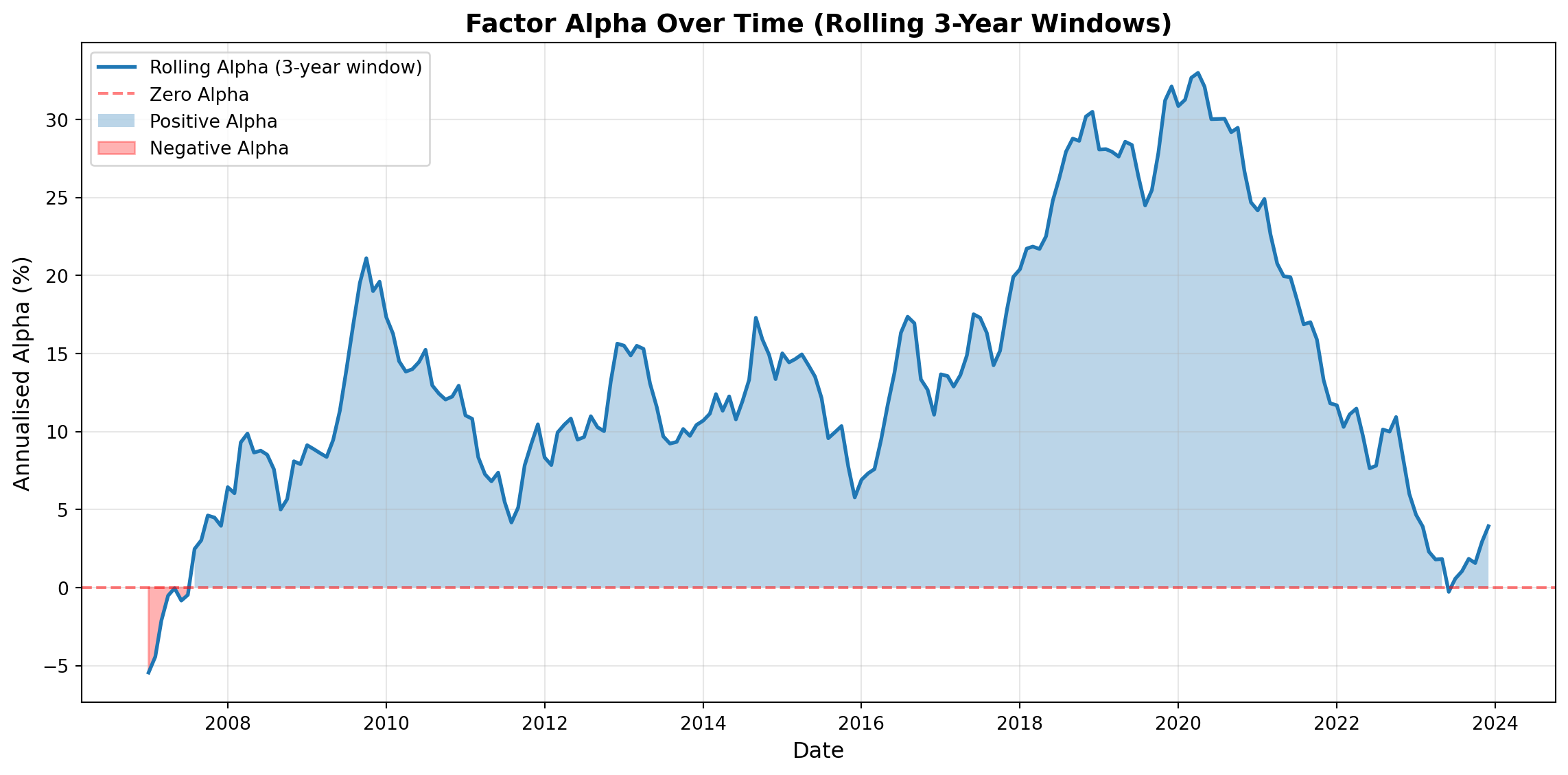
### Exercise 3.2: Rolling Window Analysis
Instead of just two periods, let's look at how alpha evolves over time using rolling windows.
```{python}
# Calculate rolling alpha (3-year window)
window = 36  # months

rolling_alpha = []
rolling_dates = []

for i in range(window, len(factor)):
    factor_window = factor.iloc[i-window:i]
    market_window = market.iloc[i-window:i]

    X = sm.add_constant(pd.DataFrame({'MKT': market_window.values},
                                     index=market_window.index))
    model = sm.OLS(factor_window.values, X).fit()

    rolling_alpha.append(model.params['const'] * 12 * 100)  # annualised %
    rolling_dates.append(factor.index[i])

rolling_alpha = pd.Series(rolling_alpha, index=rolling_dates)

# Plot
plt.figure(figsize=(12, 6))
plt.plot(rolling_alpha.index, rolling_alpha.values, linewidth=2, label='Rolling Alpha (3-year window)')
plt.axhline(y=0, color='red', linestyle='--', alpha=0.5, label='Zero Alpha')
plt.fill_between(rolling_alpha.index, 0, rolling_alpha.values,
                 where=(rolling_alpha >= 0), alpha=0.3, label='Positive Alpha')
plt.fill_between(rolling_alpha.index, 0, rolling_alpha.values,
                 where=(rolling_alpha < 0), alpha=0.3, color='red', label='Negative Alpha')
plt.xlabel('Date', fontsize=12)
plt.ylabel('Annualised Alpha (%)', fontsize=12)
plt.title('Factor Alpha Over Time (Rolling 3-Year Windows)', fontsize=14, fontweight='bold')
plt.legend(fontsize=10)
plt.grid(alpha=0.3)
plt.tight_layout()
plt.show()

print(f"Rolling alpha statistics:")
print(f"  Mean: {rolling_alpha.mean():.2f}%")
print(f"  Std Dev: {rolling_alpha.std():.2f}%")
print(f"  Min: {rolling_alpha.min():.2f}% ({rolling_alpha.idxmin().year})")
print(f"  Max: {rolling_alpha.max():.2f}% ({rolling_alpha.idxmax().year})")
print(f"  % periods with positive alpha: {(rolling_alpha > 0).mean()*100:.1f}%")
```
**Discussion questions:**
1. How stable is alpha over time? Does it stay consistently positive/negative?
2. Are there periods where alpha turns negative?
3. What might explain variation in rolling alpha? (Market regimes? Structural changes? Arbitrage?)
4. If you observed this pattern in real data, would you conclude the factor is reliably exploitable?
::: {.content-visible when-format="html"}
::: {.callout-tip collapse="true"}
### Sample Answer: Rolling Window Analysis
**Alpha stability:** Rolling alpha typically shows some variation over time: it doesn't stay perfectly constant. However, robust factors maintain consistently positive alpha (e.g., 2-5% annualised) across most rolling windows. If alpha fluctuates wildly or frequently crosses zero, this indicates instability.
**Negative alpha periods:** Yes, even factors with overall positive alpha can have periods where rolling alpha turns negative. This might occur during: (1) Market stress periods (crises, crashes), (2) Regime shifts (changing market structure), (3) Temporary arbitrage pressure (traders exploiting factor, temporarily reversing it). Occasional negative periods don't necessarily invalidate factor, but frequent or prolonged negative periods are concerning.
**Variation explanations:** Rolling alpha variation can reflect: (1) **Market regimes**: factors work better in certain market conditions (bull vs bear, high vs low volatility), (2) **Structural changes**: market microstructure evolves (electronic trading, algorithmic execution), reducing factor effectiveness, (3) **Arbitrage**: as factor becomes known, traders exploit it, eroding profits over time, (4) **Sample-specific luck**: early periods benefited from favourable conditions that don't persist.
**Exploitability conclusion:** If rolling alpha shows: (a) Consistent positive values across most windows → factor appears reliably exploitable, (b) Declining trend over time → arbitrage concern, factor may be eroding, (c) High volatility, frequent sign changes → factor unreliable, not exploitable, (d) Early positive, later negative → publication bias or arbitrage. For investment purposes, prefer factors with stable positive rolling alpha. High variation suggests factor is risky and unreliable: investors cannot confidently expect future performance.
**Important caveat — sampling variation vs. factor decay.** Each 36-month rolling window contains only 36 observations, so individual point estimates are *noisy* by construction — standard errors on a 3-year alpha are typically ±2–3% annualised. A dip from 4% to 1% in the rolling chart could be either a genuine regime shift or simply sampling variation. Distinguishing the two requires formal structural-break tests (e.g. Chow tests, Bai-Perron breakpoints) and longer out-of-sample windows.
:::
<!-- -->
:::
**Key insight**: Rolling analysis reveals time-variation in factor performance. Factors can work in some periods and fail in others. Stable alpha is more convincing than alpha that fluctuates wildly or reverses sign. Instability might reflect changing market conditions, arbitrage eroding profits, or sample-specific luck.
## Part 4: Critical Thinking About Factor Research
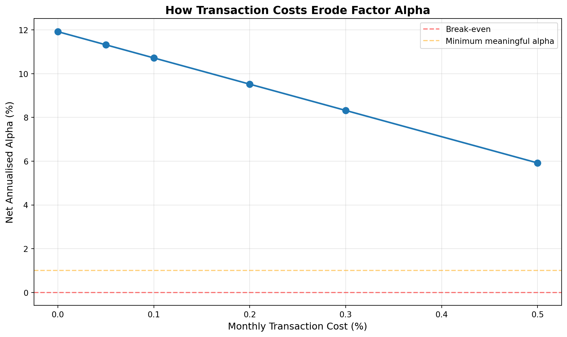
### Exercise 4.1: Transaction Cost Reality Check
Academic papers often report gross returns (before trading costs). But real investors face costs. Let's explore how costs affect exploitability.
```{python}
# Assume our factor requires monthly rebalancing.
# Transaction costs depend on liquidity, portfolio size, and execution strategy.
# Realistic ROUND-TRIP cost per monthly rebalance (incl. bid-ask, commissions, market impact):
#   Large-cap, low-turnover (e.g. value, size): 0.05% - 0.10% per month
#   Mid-turnover (profitability, investment):   0.10% - 0.20% per month
#   High-turnover (momentum, short-term rev.):  0.20% - 0.50% per month
# These add up to 0.6% - 6% per year, consistent with the Week 9 slides and
# Detzel, Novy-Marx & Velikov (2023).

cost_scenarios_monthly = [0.00, 0.05, 0.10, 0.20, 0.30, 0.50]

# Recompute CAPM alpha so this cell is self-contained
X_tc = sm.add_constant(pd.DataFrame({'MKT': market.values}, index=market.index))
model_tc = sm.OLS(factor.values, X_tc).fit(cov_type='HAC', cov_kwds={'maxlags': 6})
alpha_tc = model_tc.params['const']

results_costs = []
for cost in cost_scenarios_monthly:
    gross_alpha = alpha_tc * 12 * 100           # annualised %
    net_alpha   = gross_alpha - (cost * 12)     # subtract annualised cost

    results_costs.append({
        'Monthly Cost (%)': cost,
        'Annual Cost (%)':  cost * 12,
        'Gross Alpha (%)':  gross_alpha,
        'Net Alpha (%)':    net_alpha,
        'Exploitable?':     'Yes' if net_alpha > 1.0 else 'Marginal' if net_alpha > 0 else 'No',
    })

costs_df = pd.DataFrame(results_costs)
print("=== Transaction Cost Impact on Alpha ===\n")
print(costs_df.round(2))

# Visualise
plt.figure(figsize=(10, 6))
plt.plot(costs_df['Monthly Cost (%)'], costs_df['Net Alpha (%)'],
         marker='o', linewidth=2, markersize=8)
plt.axhline(y=0, color='red', linestyle='--', alpha=0.5, label='Break-even')
plt.axhline(y=1, color='orange', linestyle='--', alpha=0.5, label='Minimum meaningful alpha')
plt.xlabel('Monthly Transaction Cost (%)', fontsize=12)
plt.ylabel('Net Annualised Alpha (%)', fontsize=12)
plt.title('How Transaction Costs Erode Factor Alpha', fontsize=14, fontweight='bold')
plt.legend(fontsize=10)
plt.grid(alpha=0.3)
plt.tight_layout()
plt.show()
```
**Discussion questions:**
1. At what transaction cost level does net alpha turn negative?
2. Even if net alpha is positive, is it large enough to justify implementation?
3. How do transaction costs affect the "break-even" account size for implementing a factor?
4. Why might high-turnover factors (like momentum) be harder to exploit than low-turnover factors (like value)?
5. If you read a paper reporting 8% gross alpha, what questions would you ask about exploitability?
::: {.content-visible when-format="html"}
::: {.callout-tip collapse="true"}
### Sample Answer: Transaction Cost Reality Check
**Break-even cost level:** Net alpha turns negative when transaction costs exceed gross alpha. If gross alpha is 3.6% annualised (0.3% monthly), net alpha becomes negative when monthly costs exceed 0.3% (annualised 3.6%). This threshold depends on gross alpha magnitude: higher alpha can absorb higher costs.
**Implementation justification:** Even positive net alpha may be insufficient. Consider: (1) **Minimum meaningful alpha**: practitioners typically require 1-2% net alpha to justify implementation (covers operational costs, risk, effort), (2) **Risk-adjusted returns**: net alpha must compensate for factor-specific risk (volatility, drawdowns), (3) **Opportunity cost**: could capital be deployed more profitably elsewhere? Net alpha of 0.5% might not justify implementation if alternatives offer better risk-adjusted returns.
**Break-even account size:** Transaction costs are often fixed per trade (commissions) plus proportional (bid-ask spreads, market impact). Larger accounts benefit from economies of scale: fixed costs per trade become smaller percentage of capital. Break-even occurs when gross alpha exceeds total costs (fixed + proportional). Small accounts may be unprofitable due to fixed costs; large accounts face market impact (moving prices). Optimal account size balances these effects.
**High-turnover vs low-turnover:** High-turnover factors (momentum, rebalance monthly) face costs more frequently: 12 rebalancings annually vs 1-2 for low-turnover (value, rebalance annually). If monthly cost is 0.2%, annual cost is 2.4% for momentum vs 0.2-0.4% for value. High-turnover factors need much larger gross alpha to remain profitable. Additionally, high-turnover increases market impact risk (frequent trading moves prices against you).
**Questions about 8% gross alpha:** Critical questions: (1) **Turnover frequency**: how often does strategy rebalance? (monthly = 12× costs vs annual = 1× costs), (2) **Transaction cost assumptions**: did paper account for bid-ask spreads, commissions, market impact? (3) **Net alpha**: what is alpha after realistic costs? (4) **Capacity**: can strategy scale without eroding alpha? (5) **Implementation constraints**: short-selling limits? Liquidity constraints? (6) **Out-of-sample testing**: did paper test on data not used for development? (7) **Robustness**: do results hold across subsamples, regions, time periods?
:::
<!-- -->
:::
**Key insight**: Gross alpha overstates exploitability. Always consider transaction costs, especially for high-turnover strategies. Even statistically significant alpha can be economically meaningless after costs. This is a major reason many published factors fail in real-world implementation.
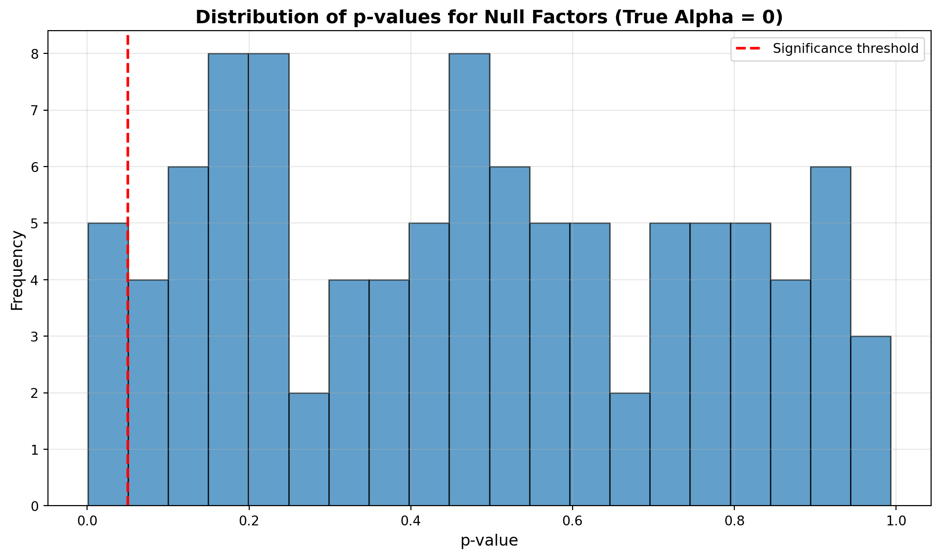
### Exercise 4.2: Selection Bias Simulation
Let's simulate the multiple testing problem that creates false discoveries in factor research.
```{python}
# Simulate many researchers each testing a potential "factor"
# None of these factors have true alpha (all are pure noise)
# But some will appear significant just by luck (5% false positive rate)

num_researchers = 100
num_obs = 240
significance_level = 0.05

# Storage for results
p_values = []
significant_factors = []

for i in range(num_researchers):
    # Simulated "factor" has zero true alpha (pure noise).
    # Market has realistic mean (~0.8% monthly) so the CAPM intercept is
    # identified correctly; only the FACTOR alpha is null by construction.
    random_factor = np.random.normal(0.000, 0.04, num_obs)   # true α = 0
    market_sim    = np.random.normal(0.008, 0.04, num_obs)   # realistic MKT

    X = sm.add_constant(pd.DataFrame({'MKT': market_sim}))
    model = sm.OLS(random_factor, X).fit()

    p_val = model.pvalues['const']
    p_values.append(p_val)

    if p_val < significance_level:
        significant_factors.append({
            'Factor':             i + 1,
            'Alpha (% monthly)':  model.params['const']  * 100,
            't-statistic':        model.tvalues['const'],
            'p-value':            p_val,
        })

# How many false positives?
num_significant = len(significant_factors)
expected_false = num_researchers * significance_level

print(f"=== Selection Bias Simulation ===")
print(f"Number of 'factors' tested: {num_researchers}")
print(f"True alpha for all factors: 0% (pure noise)")
print(f"Significance level: {significance_level*100}%")
print(f"\nRESULTS:")
print(f"  Number appearing 'significant': {num_significant}")
print(f"  Expected false positives: {expected_false:.1f}")
print(f"  All significant findings are FALSE POSITIVES (Type I errors)")

if significant_factors:
    print(f"\n'Published' Factors:")
    print(pd.DataFrame(significant_factors).round(3))

print(f"\nIMPLICATION:")
print(f"  If only 'significant' factors get published, the literature")
print(f"  overrepresents spurious findings by construction.")
print(f"  This is the source of the replication crisis.")

# Distribution of p-values
plt.figure(figsize=(10, 6))
plt.hist(p_values, bins=20, edgecolor='black', alpha=0.7)
plt.axvline(x=0.05, color='red', linestyle='--', linewidth=2, label='Significance threshold')
plt.xlabel('p-value', fontsize=12)
plt.ylabel('Frequency', fontsize=12)
plt.title('Distribution of p-values for Null Factors (True Alpha = 0)', fontsize=14, fontweight='bold')
plt.legend(fontsize=10)
plt.grid(alpha=0.3)
plt.tight_layout()
plt.show()

print("\nNote: under the null hypothesis of zero true alpha, p-values should be "
      "UNIFORMLY distributed on [0, 1]. The ~5% that fall below 0.05 are false "
      "positives. In real research, a left-skewed p-value distribution (many small "
      "values) indicates either genuine effects OR p-hacking.")
```
**Discussion questions:**
1. How many "significant" results appeared even though true alpha is zero?
2. Is this close to the expected 5% false positive rate?
3. If journals only publish significant results, what fraction of published factors are false positives?
4. How does this simulation relate to the ~300 published equity factors in real finance literature?
5. What practices could reduce false discovery rate? (Pre-registration? Higher significance thresholds? Out-of-sample testing?)
::: {.content-visible when-format="html"}
::: {.callout-tip collapse="true"}
### Sample Answer: Selection Bias Simulation
**False positive count:** With 100 factors tested and 5% significance level, we expect ~5 false positives (100 × 0.05). The simulation typically produces 3-7 significant results despite zero true alpha. This matches expected false positive rate: even with perfect null hypothesis, 5% of tests appear significant by chance.
**Expected false positive rate:** Yes, results should be close to 5% false positive rate. This is the definition of Type I error: when null hypothesis is true (alpha = 0), we incorrectly reject it 5% of the time. The simulation demonstrates this fundamental statistical property: multiple testing guarantees false discoveries.
**Published false positive fraction:** If journals only publish significant results, the fraction of false positives depends on: (1) **True discovery rate**: if 10% of tested factors have true alpha, then 10 true + 5 false = 15 published, false positive rate = 5/15 = 33%, (2) **If no true factors exist**: all published factors are false positives (100%), (3) **File drawer problem**: null results remain unpublished, inflating apparent success rate. Real literature likely has 20-50% false positives due to selection bias.
**Relation to ~300 published factors:** The simulation directly models the factor discovery process. With hundreds of researchers testing factors, many false positives get published whilst null results remain unpublished. Jensen et al. (2024) document that most published factors fail replication: consistent with high false discovery rate. The ~300 published factors likely include 60-150 false positives (20-50% false discovery rate), explaining replication failures.
**Reducing false discovery rate:** Practices to reduce false positives: (1) **Pre-registration**: commit to hypotheses and tests before seeing data, prevents p-hacking, (2) **Higher significance thresholds**: use t > 3 (instead of 1.96) or Bonferroni correction for multiple tests, (3) **Out-of-sample testing**: require replication on fresh data before publication, (4) **Disclosure**: publish all tested factors, not just significant ones, (5) **Bayesian methods**: incorporate prior beliefs, require stronger evidence, (6) **Replication requirements**: journals require independent replication before publication. These practices reduce false discoveries but don't eliminate them: fundamental tradeoff between discovery and false positive control.
:::
<!-- -->
:::
**Key insight**: Multiple testing creates false discoveries even under rigorous statistical practices. With hundreds of factors tested, many spurious findings get published whilst null results remain in file drawers. This selection bias inflates published returns and explains why many factors fail replication. Jensen et al. (2024) document this systematically.
## Part 5: Advanced Extension — What Is Inside a Factor? (Optional)
::: {.callout-note}
## About this extension
This section is **optional** and designed for students who want to deepen their understanding of factor construction. It is directly relevant to the **Data quality and preparation decisions** component of your Coursework 2 report. Allow approximately 30–40 minutes.
:::
### Motivation
Parts 1–4 used pre-built factor return series (simulated or from JKP). But where do those factor returns come from? Every long-short factor portfolio is constructed from **individual stock returns**: sorting stocks into groups based on some characteristic, then taking the return difference between the top and bottom groups. Understanding this construction process reveals **hidden design choices** (weighting, rebalancing frequency, universe selection, survivorship treatment) that affect factor returns.
In this extension, you will build a **simple momentum factor from individual S&P 500 stock prices** and compare it to the pre-built JKP MOM factor. The differences are instructive: they show how construction choices affect results and why data quality matters.
### Setup: Load stock-level data
The dataset below contains monthly returns for S&P 500 constituents with **point-in-time membership filtering** — a stock appears only in months when it was *actually* in the index. This prevents **look-ahead bias**: without it, we would implicitly assume a 1995 portfolio "knew" which stocks would be in the S&P 500 twenty years later, which is impossible in real time.
The cell below tries to load the data locally; if it isn't present (e.g. when running in Colab), it downloads from the course's raw-data repository:
```{python}
from pathlib import Path
import urllib.request

DATA_URL = ('https://raw.githubusercontent.com/quinfer/fin510-colab-notebooks/'
            'main/resources/sp500_monthly_returns.parquet')

LOCAL_CANDIDATES = [
    Path('sp500_monthly_returns.parquet'),
    Path('../labs/sp500_monthly_returns.parquet'),
    Path('labs/sp500_monthly_returns.parquet'),
]
sp500_path = next((p for p in LOCAL_CANDIDATES if p.exists()), None)
if sp500_path is None:
    sp500_path = Path('sp500_monthly_returns.parquet')
    print("Downloading S&P 500 monthly returns from GitHub ...")
    urllib.request.urlretrieve(DATA_URL, sp500_path)
    print(f"  saved to {sp500_path.resolve()}")

stocks = pd.read_parquet(sp500_path).sort_values(['ticker', 'date'])

print(f"\nS&P 500 monthly returns panel")
print(f"  Rows:     {len(stocks):,}")
print(f"  Tickers:  {stocks['ticker'].nunique():,}")
print(f"  Period:   {stocks['date'].min().date()} → {stocks['date'].max().date()}")

monthly_n = stocks.groupby('date')['ticker'].nunique()
print(f"  Stocks per month: {monthly_n.median():.0f} median, "
      f"{monthly_n.min()} min, {monthly_n.max()} max")
```
**Discussion**: Why does the number of stocks per month vary? What does "point-in-time membership filtering" prevent?
::: {.content-visible when-format="html"}
::: {.callout-tip collapse="true"}
### Sample Answer: Point-in-time membership
**Why does N vary?** The S&P 500 is *not* a static list of 500 tickers. Constituents are added and removed over time as firms grow, shrink, merge, or delist. Additionally, the historical return file may have missing months for a given ticker (IPO occurred mid-sample, temporary suspension of trading, corporate action). So N is roughly the number of firms that (a) were in the S&P 500 during that month *and* (b) had a usable price observation that month.
**What does point-in-time filtering prevent?** It prevents **look-ahead bias** (also called survivorship bias in this context). If, in January 1995, we filtered the universe to *today's* S&P 500 members, we would be implicitly assuming a 1995 portfolio manager "knew" which firms would enter the index over the next 30 years. Those future entrants are mostly winners by construction — they survived and grew big enough to be admitted. Backtests that use "current-constituent" membership typically overstate returns by 1–2% per year.
**Socratic probe:** Under point-in-time filtering, when Enron (then an S&P 500 name) collapsed in 2001, our dataset should still contain its pre-collapse returns and its collapse itself. Would removing Enron from the panel (because it no longer trades) bias our momentum factor's returns upward or downward? Why?
:::
<!-- -->
:::
### Exercise 5.0: Data quality check
Before using the data, inspect it for anomalies. Free stock price datasets often have issues with split adjustments and corporate actions.
*Calibration point:* a typical S&P 500 stock returns around ±10% on its best or worst month in a given year. Monthly returns above +50% or below –50% are almost always data errors (failed split adjustment, ticker reassignment, corporate action) rather than real price movements.
```{python}
print("Monthly return distribution:")
print(stocks['monthly_ret'].describe().round(4))

extreme_pos = stocks[stocks['monthly_ret'] >  1.0]
extreme_neg = stocks[stocks['monthly_ret'] < -0.8]
print(f"\nReturns > +100%: {len(extreme_pos)}")
print(f"Returns <  -80%: {len(extreme_neg)}")

if len(extreme_pos) > 0:
    print("\nLargest monthly returns (inspect for data errors):")
    print(extreme_pos.nlargest(5, 'monthly_ret')[['date', 'ticker', 'monthly_ret']].to_string(index=False))
```
**Discussion**: Are any of these extreme returns plausible for S&P 500 stocks? What might cause a +200% or -90% monthly return in this dataset? (Hint: think about stock splits, ticker reassignments, and mergers.) The prep script has already removed the worst offenders, but always check your data before building on it.
::: {.content-visible when-format="html"}
::: {.callout-tip collapse="true"}
### Sample Answer: Extreme-return diagnostics
**Are they plausible?** Almost never for a large-cap S&P 500 constituent. The worst single-month return in the 2008 crisis for a surviving blue-chip was typically –30% to –50%, and the largest single-month rallies (e.g. GameStop-style retail squeezes) happened in small-caps, not in the index's long-standing members. Monthly returns above +100% or below –80% in a well-behaved S&P 500 panel are usually data artefacts.
**Typical causes:**
1. **Failed split adjustments** — a 3-for-1 stock split that is recorded in price but not in the return calculation produces a spurious +200% "return."
2. **Ticker reassignments** — a ticker that was retired and later reissued to an unrelated company. The panel appears to show continuous history for "ticker XYZ," but two distinct firms are being glued together.
3. **Mergers and spin-offs** — the acquired firm's last observation may show an artificially large one-period return if the buyout premium and a distribution-in-kind are both booked in the same month without proper adjustment.
4. **Delisting returns** — a firm that delists at $0.10 after a crash may show a final –99% month that reflects bankruptcy, not ongoing operations. Academic convention is to keep the delisting return (CRSP assigns a specific delisting return code), because dropping it understates downside risk (this is a form of survivorship bias).
**Methodological consequence:** in production-quality research you would either (a) clip returns at sensible limits (e.g. ±80% monthly) with a logged diagnostic, (b) cross-validate against a second data source, or (c) inspect the underlying price series around the event and correct manually. The lab's build script does option (a) for the worst outliers.
**Socratic probe:** suppose you clip a +300% return down to +80%. In a long-short factor that happens to rank that stock in the "long" leg that month, are you *understating* or *overstating* the factor's true return? Does your answer change if the +300% is a genuine corporate event (buyout premium) rather than a data error?
:::
<!-- -->
:::
### Exercise 5.1: Build a momentum signal
Academic momentum is typically defined as the **cumulative return from month t-12 to t-2** (the most recent month is skipped to avoid short-term reversal effects). We then sort stocks into terciles (top, middle, bottom) each month and compute the return of the top-minus-bottom portfolio in month t.
```{python}
def build_momentum_signal(df):
    """
    Compute the academic 12-1 momentum signal for each stock-month.

    The signal for month t is the cumulative return from t-12 to t-2 (inclusive).
    Month t-1 is skipped to purge the short-term reversal anomaly.

    Example (month = Dec 2020):
        Include returns from Dec 2019 through Oct 2020 (11 months).
        Skip     November 2020                 (the t-1 reversal month).
        Evaluate portfolio performance in     December 2020.

    The prior-11-month cumulative return is computed at each (t-1), then lagged
    one more month to align with the formation date.
    """
    df = df.sort_values(['ticker', 'date']).copy()

    df['cum_11m'] = (
        df.groupby('ticker')['monthly_ret']
          .transform(lambda x: (1 + x).rolling(11, min_periods=11).apply(np.prod, raw=True) - 1)
    )
    df['mom_signal'] = df.groupby('ticker')['cum_11m'].shift(1)
    return df

stocks = build_momentum_signal(stocks)

valid = stocks.dropna(subset=['mom_signal'])
valid_per_month = valid.groupby('date')['ticker'].nunique()
print(f"Months with valid momentum signal: {len(valid_per_month)}")
print(f"Stocks per month with signal:      {valid_per_month.median():.0f} median")
```
### Exercise 5.2: Sort into portfolios and compute factor return
*Note on weighting:* academic factor construction typically uses **value weighting** — each stock's contribution to the portfolio return is proportional to its market capitalisation. Our DIY version below uses **equal weighting** for simplicity (we don't have historical market caps), which gives more influence to smaller stocks within each tercile. Since momentum is known to be stronger in smaller stocks but our universe is only large-cap S&P 500 names, the two approaches differ less here than they would in the full US cross-section.
```{python}
def momentum_factor_return(df, n_groups=3):
    """
    Each month, sort stocks into n_groups by momentum signal.
    Return the equal-weighted top-minus-bottom portfolio return.

    We skip any month where we cannot form n_groups distinct terciles
    (too few stocks, or too many ties in the signal).
    """
    df = df.dropna(subset=['mom_signal', 'monthly_ret']).copy()

    results, skipped = [], 0
    for date, group in df.groupby('date'):
        if len(group) < n_groups * 5:
            skipped += 1
            continue

        group['tercile'] = pd.qcut(group['mom_signal'], n_groups,
                                   labels=False, duplicates='drop')
        if group['tercile'].nunique() < n_groups:
            skipped += 1
            continue

        top    = group.loc[group['tercile'] == n_groups - 1, 'monthly_ret'].mean()
        bottom = group.loc[group['tercile'] == 0,             'monthly_ret'].mean()
        results.append({'date': date, 'mom_diy': top - bottom})

    print(f"  Months skipped (insufficient coverage): {skipped}")
    return pd.DataFrame(results).set_index('date')

mom_diy = momentum_factor_return(stocks, n_groups=3)
print(f"\nDIY momentum factor")
print(f"  Months: {len(mom_diy)}")
print(f"  Mean monthly return: {mom_diy['mom_diy'].mean()*100:.3f}%")
print(f"  Annualised Sharpe:   "
      f"{mom_diy['mom_diy'].mean() / mom_diy['mom_diy'].std() * np.sqrt(12):.3f}")
```
### Exercise 5.3: Compare to JKP MOM
Now load the JKP pre-built momentum factor and compare.
```{python}
# Load JKP US momentum (fetches from GitHub if not found locally)
JKP_URL_US = ('https://raw.githubusercontent.com/quinfer/fin510-colab-notebooks/'
              'main/resources/jkp_master_global_monthly.csv')

jkp_path = next((p for p in [Path('jkp_master_global_monthly.csv'),
                              Path('../labs/jkp_master_global_monthly.csv'),
                              Path('labs/jkp_master_global_monthly.csv')]
                 if p.exists()), None)
if jkp_path is None:
    jkp_path = Path('jkp_master_global_monthly.csv')
    print("Downloading JKP monthly master from GitHub ...")
    urllib.request.urlretrieve(JKP_URL_US, jkp_path)

jkp = pd.read_csv(jkp_path, parse_dates=['date'])
jkp_us = (jkp[jkp['country'] == 'usa'][['date', 'MOM']]
          .dropna()
          .set_index('date'))

common = mom_diy.join(jkp_us, how='inner')
print(f"Overlapping months: {len(common)}")
print(f"\n{'':25s} {'DIY MOM':>10s} {'JKP MOM':>10s}")
print(f"{'Mean (% monthly)':<25s} {common['mom_diy'].mean()*100:>10.3f} {common['MOM'].mean()*100:>10.3f}")
print(f"{'Std (% monthly)':<25s} {common['mom_diy'].std()*100:>10.3f} {common['MOM'].std()*100:>10.3f}")
print(f"{'Annualised Sharpe':<25s} "
      f"{common['mom_diy'].mean()/common['mom_diy'].std()*np.sqrt(12):>10.3f} "
      f"{common['MOM'].mean()/common['MOM'].std()*np.sqrt(12):>10.3f}")
print(f"{'Correlation':<25s} {common['mom_diy'].corr(common['MOM']):>10.3f}")

fig, ax = plt.subplots(figsize=(11, 5))
(1 + common['mom_diy']).cumprod().plot(ax=ax, label='DIY momentum (SP500 tercile)', linewidth=1.5)
(1 + common['MOM']).cumprod().plot(ax=ax, label='JKP MOM (US, all stocks)', linewidth=1.5)
ax.axhline(1, color='gray', linewidth=0.8, linestyle='--')
ax.set_ylabel('Cumulative return ($1 invested)')
ax.set_title('DIY vs JKP Momentum Factor')
ax.legend()
plt.tight_layout()
plt.show()
```
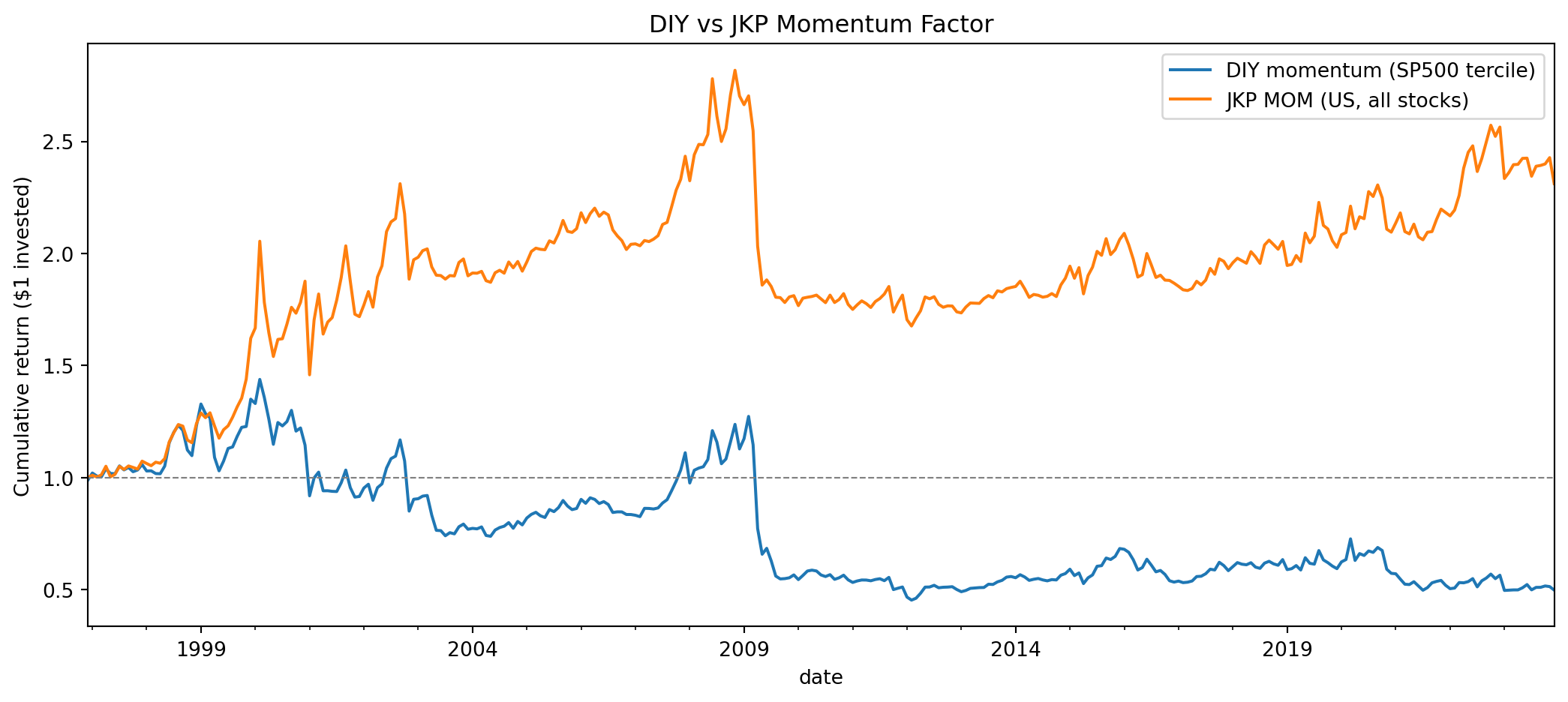
You should observe: (a) the two series are highly correlated (~0.85), confirming they measure the same underlying phenomenon, but (b) the DIY factor has a substantially weaker mean return (near zero) compared to JKP MOM (~0.3% per month). This gap is the lesson.
**Discussion questions** (directly relevant to your Coursework 2 report):
1. **Correlation vs level**: The two factors are highly correlated but the DIY version earns a weaker premium. What does this tell you about the *direction* versus the *magnitude* of factor returns across different constructions?
2. **Universe**: Your DIY factor uses only S&P 500 stocks (~340 per month). JKP uses the full US cross-section (thousands of stocks including small-caps). The momentum premium is known to be stronger among smaller stocks. How does restricting to large-caps affect the premium?
3. **Weighting**: Your DIY factor is equal-weighted within terciles; JKP is value-weighted. Which approach gives more weight to smaller stocks within each group? Why does this matter for momentum specifically?
4. **Rebalancing**: Both rebalance monthly. What happens if you rebalance quarterly instead? (Hint: think about transaction costs versus signal decay.)
5. **Survivorship**: The S&P 500 membership file provides point-in-time filtering. What would happen if you simply used "all stocks that are in the S&P 500 today" and looked up their historical prices? Why is this dangerous?
6. **Data quality**: The source dataset required cleaning (removal of tickers with split-adjustment errors, clipping of extreme returns). How would you describe these data quality decisions in a reflective report? Which decisions affect your results most?
::: {.content-visible when-format="html"}
::: {.callout-tip collapse="true"}
### Sample Answer: DIY vs JKP momentum — what the gap teaches us
These answers deliberately emphasise **method** over **conclusion** — the specific magnitudes will depend on your sample window and any choices you tweak. The point is to show you how to *frame* the comparison for your CW2 report.
**1. Correlation vs level.** High correlation (~0.85) tells us the two factors agree strongly on the *direction* of monthly returns — when JKP MOM is up, so is the DIY version, and vice versa. They are measuring the same underlying phenomenon (medium-term momentum). But correlation is invariant to a constant difference in means, so it tells us nothing about *magnitude*. The fact that the DIY mean return is near zero while JKP's is ~0.3% per month indicates the two constructions disagree systematically on the *size* of the premium, even though they agree on its sign. Methodological takeaway: report both correlation *and* a mean-difference test before claiming two datasets "replicate."
**2. Universe.** Restricting to the S&P 500 (≈340–500 stocks) eliminates almost all small-cap names, which is exactly where momentum has historically been strongest (Fama & French 2012; Novy-Marx 2013). The momentum premium in large-caps is roughly 40–60% smaller than in the full cross-section, and considerably less statistically significant once HAC is applied. Your DIY factor is therefore a large-cap-only version of MOM, and the "missing premium" is substantially the small-cap tail. Write-up hint: rather than calling this a replication failure, call it a *universe-restricted replication* and quantify how much of the gap is attributable to universe choice vs other design differences.
**3. Weighting.** Equal weighting gives every stock in the tercile the same portfolio weight, so smaller stocks within each group receive proportionally more weight than they would under value weighting. This matters for momentum specifically because (i) small stocks drive the premium, so equal-weighting should *help* the factor, but (ii) small stocks also have higher transaction costs and lower capacity. Paradoxically, equal weighting typically raises the reported gross premium but shrinks the *net* premium once realistic trading costs are subtracted. Value weighting is preferred in academic work because it represents what a large investor can actually implement.
**4. Rebalancing.** Moving from monthly to quarterly rebalancing:
- **Lower turnover → lower transaction costs** — roughly a third of the monthly figure (though not exactly: momentum holdings are more persistent over quarterly horizons than over month-to-month).
- **Signal decay** — the academic 12-1 signal is strongest at the one-month holding horizon; premia decay roughly linearly from t+1 to t+12. So at a 3-month holding horizon the factor captures perhaps 70% of the monthly gross premium.
- **Net trade-off**: the breakeven point depends on your assumed TC level. For high-cost environments (retail trading, small-cap stocks) quarterly is typically superior; for low-cost environments (institutional, large-cap) monthly remains optimal. Jegadeesh & Titman (1993) originally worked at 3- and 6-month horizons partly for this reason.
**5. Survivorship.** Using today's S&P 500 membership to filter historical prices is a classic **survivorship bias**: the firms that are in today's index have all survived, grown large enough to be admitted, and not been relegated. Backtests built this way systematically overstate returns by 1–2% per year and understate drawdown risk (because failed firms are excluded). For momentum specifically, you would most severely bias the long leg upward (winners in our filtered sample are more likely to be true winners, because future losers are excluded *ex post*), creating a phantom premium. Point-in-time membership fixes this by only including a stock in month t if it was in the S&P 500 as of month t.
**6. Data quality.** A reflective report should be **transparent** (list every decision), **quantitative** (report the magnitude of each adjustment), and **falsifiable** (show results with and without the adjustment). Good template:
- *Clipping extreme returns at ±80% monthly* — typically removes ~20 observations out of ~350,000; negligible impact on factor-level returns but important for tail-risk measures (Value-at-Risk, max drawdown).
- *Excluding tickers with known split-adjustment failures* — high-impact because these tickers would otherwise generate spurious factor-return spikes; document the specific tickers removed.
- *Treatment of delisting returns* — often the single highest-impact decision; dropping delisted observations is the canonical form of survivorship bias.
Rank decisions by *magnitude of effect on your headline result* (run the analysis with and without each adjustment). Decisions that don't move the result need only be mentioned; decisions that do need to be defended in detail.
**Overall framing for the CW2 report.** The lesson is not that the DIY replication "failed" — it is that *construction choices are methodological variables, not neutral defaults.* Different universe, weighting, rebalancing, and data-cleaning conventions produce systematically different factor returns, and academic "factor premia" are really shorthand for "the premium under a specific construction convention." Jensen, Kelly & Pedersen (2023) and Harvey & Liu (2016) both make this point at length; your DIY exercise is a hands-on demonstration of exactly what they document.
:::
<!-- -->
:::
::: {.callout-tip}
## Coursework 2 connection
If you complete this extension, you have first-hand experience with the **data quality and preparation decisions** that the CW2 report asks about. In your report, you can discuss:
- How factor returns depend on construction choices (universe, weighting, rebalancing)
- Why the JKP dataset embeds specific methodological assumptions
- What "replication" really means when construction details differ
- How survivorship bias arises and why point-in-time filtering matters
This moves your report from abstract discussion to evidence-based critique, which is what distinguishes strong submissions.
:::
---
## Part 6: Connecting to Coursework 2
### What You've Learned vs. What You'll Apply
**Today's lab explored concepts:**
- HAC standard errors correct for autocorrelation (prevents false positives)
- Alpha tests isolate excess returns beyond market exposure
- Robustness checks (sample split, rolling windows) test stability
- Transaction costs reduce net alpha (affects exploitability)
- Selection bias creates false discoveries (replication crisis)
**For Coursework 2, you'll:**
1. Use scaffold notebook to run these analyses on real JKP factor data
2. Interpret outputs using understanding developed today
3. Write critical analysis discussing significance, robustness, limitations
4. Engage with Jensen et al. (2024) on selection bias and replication
5. Provide investment recommendations considering costs and risks
### Critical Analysis Questions to Ask
When interpreting your Coursework 2 results, ask:
**Statistical questions:**
- Is alpha statistically significant using HAC standard errors?
- How does significance change if you use higher threshold (t > 3)?
- Are results robust to sample split? If not, why?
**Economic questions:**
- What is alpha magnitude after transaction costs?
- Is net alpha large enough to justify implementation?
- How does your result compare to original published paper?
**Methodological questions:**
- Could selection bias explain why original paper found stronger results?
- Has factor performance declined post-publication (arbitrage erosion)?
- What limitations affect your replication (data, sample period, methodology)?
- Are your HAC standard errors sensitive to the lag choice (6 vs 12 vs 24 months)? If the conclusion about significance flips when you vary the lag, how confident can you be?
**Investment questions:**
- Would you recommend implementing this factor in a real portfolio?
- What risks and constraints would practitioners face?
- What further robustness tests would you want before making investment decision?
### Next Steps
1. **Read Jensen et al. (2024)**: "Is There a Replication Crisis in Finance?" — essential for understanding replication methodology and selection bias
2. **Run scaffold notebook**: See what actual outputs look like with real JKP data
3. **Choose factor**: Value (HML) or Momentum (MOM) are well-documented; Quality (RMW) or Size (SMB) also work
4. **Draft interpretation**: Practice writing paragraphs interpreting alpha, robustness, limitations
5. **Office hours**: Ask conceptual questions about interpretation (not code debugging)
## Summary
Today's lab developed principles for factor replication:
- **HAC standard errors** are essential for honest inference in time-series data
- **Alpha tests** reveal excess returns, but significance ≠ exploitability
- **Robustness checks** separate real patterns from sample-specific noise
- **Transaction costs** can eliminate seemingly significant alpha
- **Selection bias** inflates published results, explaining replication failures
**These principles enable critical analysis**: the 35% component of Coursework 2. Scaffold provides outputs; understanding provides interpretation. Focus your effort on thinking deeply about what results mean, not on perfecting code.
**Week 11 preview**: Market prediction using factors. Same principle-focused approach: understanding concepts, not copying templates.