---
title: "Lab 3: Time Series Foundations"
subtitle: "Stationarity, ARIMA, and Forecasting with Bloomberg Data"
author: "Financial Data Science"
format:
html:
toc: true
toc-depth: 3
code-fold: show
code-tools: true
execute:
warning: false
message: false
---
::: {.callout-note}
### Lab Versions
This is the **homework** lab using pre-collected Bloomberg data. For the **in-class** Bloomberg Terminal session (extract SPY and VIX yourself), see [Lab 3: SPY and VIX Extraction](lab03_time_series_bloomberg.qmd).
:::
## Learning Objectives
By the end of this lab, you will be able to:
1. Test time series for stationarity using visual and statistical methods
2. Interpret ACF and PACF plots to identify AR/MA patterns
3. Fit ARIMA models to financial data
4. Perform walk-forward validation for time series forecasts
5. Compare forecast accuracy across different models
## Setup
```{python}
#| label: setup
import pandas as pd
import numpy as np
import matplotlib.pyplot as plt
import seaborn as sns

# Time series tools
import statsmodels.api as sm
from statsmodels.tsa.stattools import adfuller, kpss, acf, pacf
from statsmodels.tsa.arima.model import ARIMA
from statsmodels.graphics.tsaplots import plot_acf, plot_pacf

# Validation
from sklearn.model_selection import TimeSeriesSplit
from sklearn.metrics import mean_absolute_error, mean_squared_error

# Settings
plt.style.use('seaborn-v0_8-darkgrid')
sns.set_palette("husl")
np.random.seed(42)

# Data root (config/data_root.yml or repo data/)
from pathlib import Path
import yaml
try:
    with open(Path("config/data_root.yml")) as f:
        cfg = yaml.safe_load(f)
    data_root = Path(cfg.get("data_root", "data")).expanduser().resolve()
except Exception:
    data_root = Path("data")

# Shared Bloomberg loader (course repo: scripts/; Colab sister repo: resources/)
import sys
for _root in (
    Path("scripts"),
    Path("../scripts"),
    Path("resources"),
    Path("../resources"),
):
    _p = _root.resolve()
    if _p.is_dir() and (_p / "bloomberg_loader.py").exists():
        sys.path.insert(0, str(_p))
        break
from bloomberg_loader import load_bloomberg
```
## Part 1: Stationarity Diagnostics
### 1.1 Load Bloomberg Database
```{python}
#| label: load-data
try:
    df = load_bloomberg()
except FileNotFoundError:
    COLAB_DB_URL = "https://raw.githubusercontent.com/quinfer/fin510-colab-notebooks/main/resources/bloomberg_database.parquet"
    df = pd.read_parquet(COLAB_DB_URL)

# Preview
print(df.head())
print(f"\nAssets available: {df['ticker'].unique()}")
print(f"Date range: {df['date'].min()} to {df['date'].max()}")
```
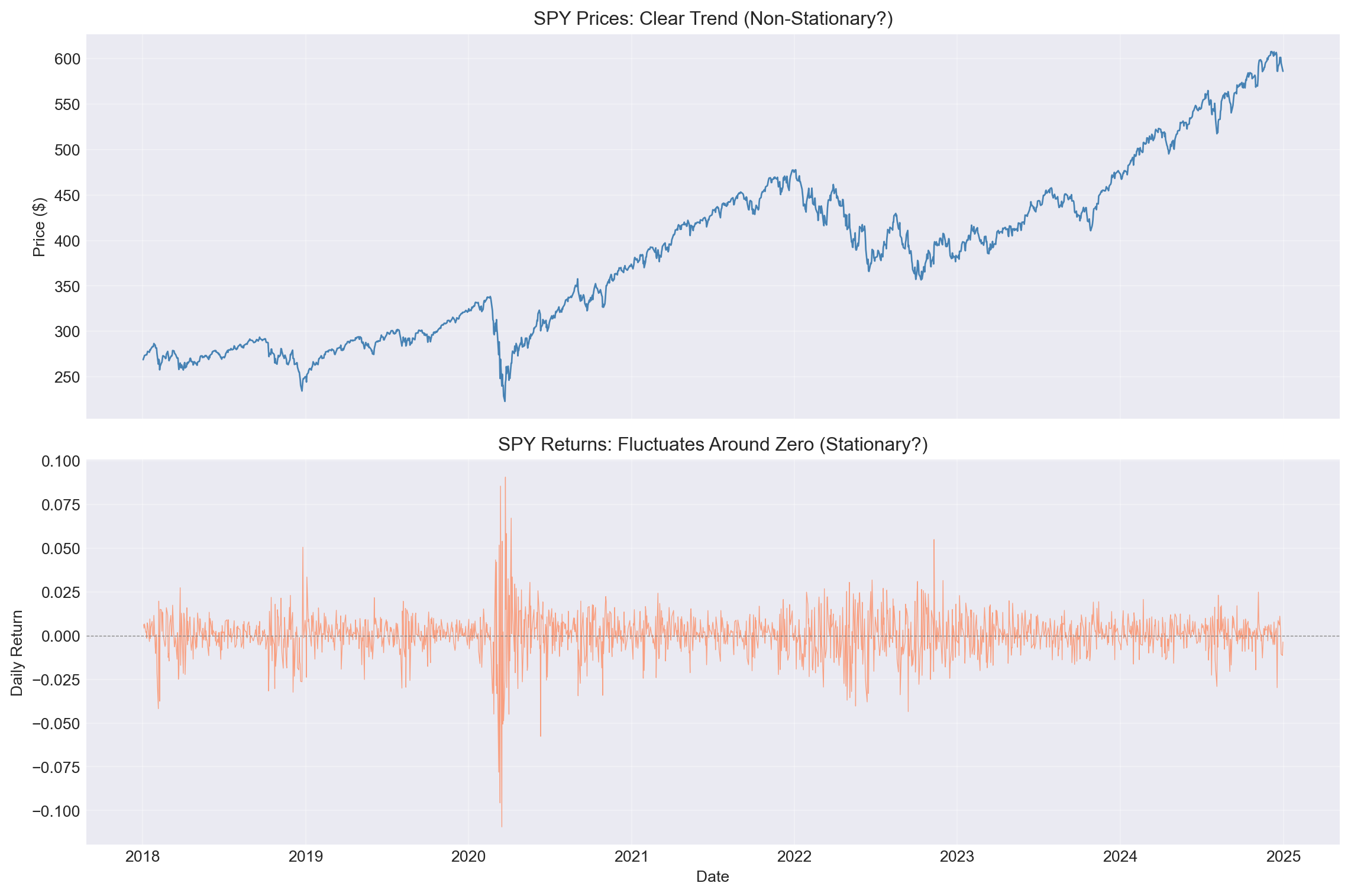
### 1.2 Visual Inspection: Prices vs Returns
**Task:** Compare SPY prices and returns to diagnose stationarity.
```{python}
#| label: spy-visual
# Extract SPY data
spy = df[df['ticker'] == 'SPY'].set_index('date').sort_index()

# Calculate returns (already in data, but let's recalculate for clarity)
spy['return'] = spy['PX_LAST'].pct_change()

# Plot prices and returns
fig, axes = plt.subplots(2, 1, figsize=(12, 8), sharex=True)

# Prices
axes[0].plot(spy.index, spy['PX_LAST'], linewidth=1, color='steelblue')
axes[0].set_ylabel('Price ($)')
axes[0].set_title('SPY Prices: Clear Trend (Non-Stationary?)')
axes[0].grid(alpha=0.3)

# Returns
axes[1].plot(spy.index, spy['return'], linewidth=0.5, color='coral', alpha=0.7)
axes[1].axhline(0, color='gray', linestyle='--', linewidth=0.5)
axes[1].set_ylabel('Daily Return')
axes[1].set_xlabel('Date')
axes[1].set_title('SPY Returns: Fluctuates Around Zero (Stationary?)')
axes[1].grid(alpha=0.3)

plt.tight_layout()
plt.show()
```
::: {.callout-note}
## Question 1.1
Based on visual inspection alone:
- Do SPY prices appear stationary? Why or why not?
- Do SPY returns appear stationary? Why or why not?
:::
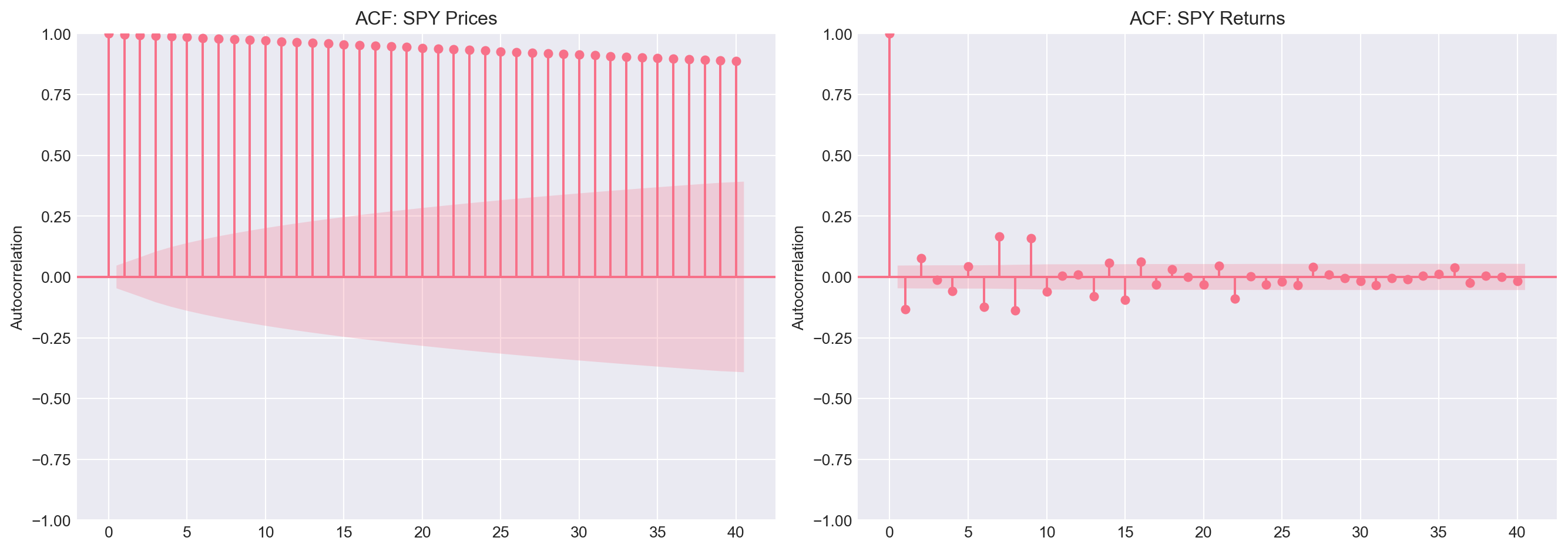
### 1.3 ACF Diagnostic
The Autocorrelation Function (ACF) provides evidence for stationarity:
- **Stationary**: ACF drops quickly to zero
- **Non-stationary**: ACF decays slowly
```{python}
#| label: spy-acf
fig, axes = plt.subplots(1, 2, figsize=(14, 5))

# ACF of prices
plot_acf(spy['PX_LAST'].dropna(), ax=axes[0], lags=40, title='ACF: SPY Prices')
axes[0].set_ylabel('Autocorrelation')

# ACF of returns
plot_acf(spy['return'].dropna(), ax=axes[1], lags=40, title='ACF: SPY Returns')
axes[1].set_ylabel('Autocorrelation')

plt.tight_layout()
plt.show()
```
::: {.callout-note}
## Question 1.2
- Which ACF plot shows slow decay?
- Which ACF plot shows rapid decay to zero?
- What does this tell you about stationarity?
:::
### 1.4 Augmented Dickey-Fuller Test
The ADF test formalises the stationarity check:
- **Null hypothesis**: Series has a unit root (non-stationary)
- **Alternative**: Series is stationary
- **Decision**: If p-value < 0.05, reject null → series is stationary
```{python}
#| label: spy-adf
def adf_test(series, name):
    """Perform ADF test and print results"""
    result = adfuller(series.dropna())
    print(f"\nADF Test: {name}")
    print("=" * 50)
    print(f"ADF Statistic: {result[0]:.4f}")
    print(f"p-value: {result[1]:.4f}")
    print(f"Critical Values:")
    for key, value in result[4].items():
        print(f"  {key}: {value:.4f}")

    if result[1] < 0.05:
        print(f"✓ Conclusion: {name} is STATIONARY (reject null at 5%)")
    else:
        print(f"✗ Conclusion: {name} is NON-STATIONARY (fail to reject null)")
    return result

# Test prices
adf_prices = adf_test(spy['PX_LAST'], "SPY Prices")

# Test returns
adf_returns = adf_test(spy['return'], "SPY Returns")
```
::: {.callout-note}
## Question 1.3
- Do the ADF test results confirm your visual intuition?
- Why is the p-value for returns much smaller than for prices?
:::
### 1.5 Exercise: Test VIX for Stationarity
**Your task:** Apply the same diagnostics to the VIX index.
```{python}
#| label: vix-exercise
# Extract VIX data
vix = df[df['ticker'] == 'VIX'].set_index('date').sort_index()

# YOUR CODE HERE:
# 1. Plot VIX over time
# 2. Plot ACF
# 3. Run ADF test
# 4. Interpret results: Is VIX stationary?

# Solution (uncomment to run):
# fig, axes = plt.subplots(2, 1, figsize=(12, 8))
#
# # Time plot
# axes[0].plot(vix.index, vix['PX_LAST'], linewidth=0.8, color='coral')
# axes[0].axhline(vix['PX_LAST'].mean(), color='steelblue', linestyle='--',
#                 label=f'Mean: {vix["PX_LAST"].mean():.1f}')
# axes[0].set_ylabel('VIX Level')
# axes[0].set_title('VIX: Mean-Reverting but Clustered')
# axes[0].legend()
# axes[0].grid(alpha=0.3)
#
# # ACF
# plot_acf(vix['PX_LAST'].dropna(), ax=axes[1], lags=40, title='ACF: VIX')
# axes[1].set_xlabel('Lag')
#
# plt.tight_layout()
# plt.show()
#
# # ADF test
# adf_test(vix['PX_LAST'], "VIX")
```
::: {.callout-tip}
## Hint
VIX is bounded (can't go negative, rarely exceeds 80) and mean-reverting, but it shows persistence. The ADF test result may be borderline.
:::
## Part 2: ACF and PACF Interpretation
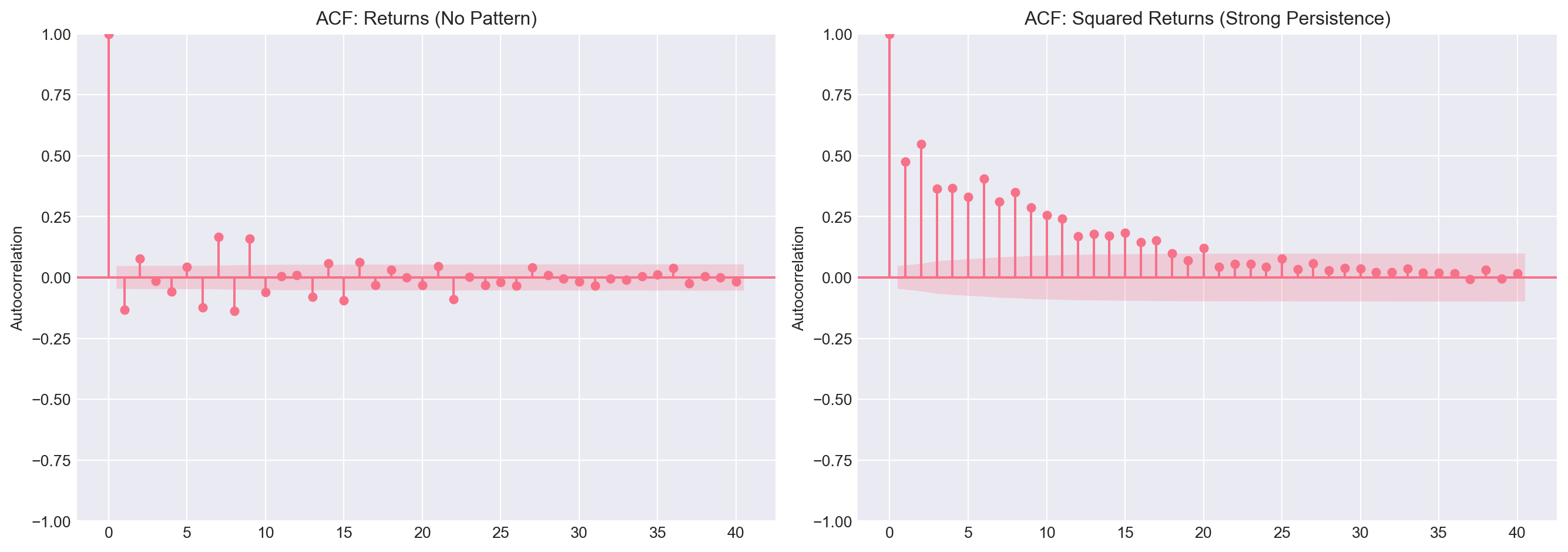
### 2.1 Volatility Clustering Preview
Remember from the slides: returns are unpredictable, but **volatility** is predictable.
```{python}
#| label: volatility-clustering
spy['return_sq'] = spy['return'] ** 2

fig, axes = plt.subplots(1, 2, figsize=(14, 5))

# ACF of returns
plot_acf(spy['return'].dropna(), ax=axes[0], lags=40, title='ACF: Returns (No Pattern)')
axes[0].set_ylabel('Autocorrelation')

# ACF of squared returns
plot_acf(spy['return_sq'].dropna(), ax=axes[1], lags=40,
         title='ACF: Squared Returns (Strong Persistence)')
axes[1].set_ylabel('Autocorrelation')

plt.tight_layout()
plt.show()
```
::: {.callout-note}
## Question 2.1
- Why do returns show no autocorrelation?
- Why do **squared** returns show strong autocorrelation?
- What does this tell you about market efficiency vs volatility?
:::
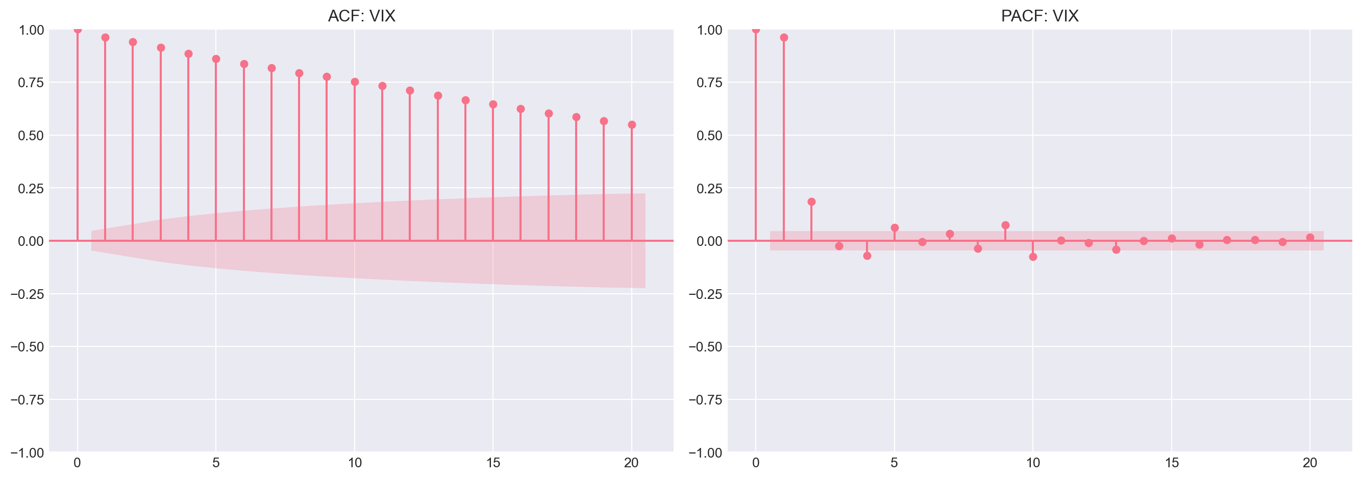
### 2.2 PACF: Identifying AR vs MA
The **Partial ACF** isolates direct lag effects.
**Interpretation rules:**
| Process | ACF Pattern | PACF Pattern |
|---------|-------------|--------------|
| AR(p) | Exponential decay | Cuts off after lag p |
| MA(q) | Cuts off after lag q | Exponential decay |
| ARMA(p,q) | Both decay | Both decay |
```{python}
#| label: vix-acf-pacf
fig, axes = plt.subplots(1, 2, figsize=(14, 5))

# ACF
plot_acf(vix['PX_LAST'].dropna(), ax=axes[0], lags=20, title='ACF: VIX')

# PACF
plot_pacf(vix['PX_LAST'].dropna(), ax=axes[1], lags=20, title='PACF: VIX')

plt.tight_layout()
plt.show()
```
::: {.callout-note}
## Question 2.2
Looking at the VIX ACF and PACF:
- Does the PACF cut off sharply after lag 1?
- Does the ACF decay gradually?
- What does this pattern suggest? (Hint: AR process)
:::
## Part 3: Fitting ARIMA Models
The standard workflow is the **Box–Jenkins approach**: (1) identify order using ACF/PACF, (2) estimate the model, (3) diagnose residuals (check for white noise). If residuals show autocorrelation, consider more lags or a different specification (Brooks, 2019, Ch 5).
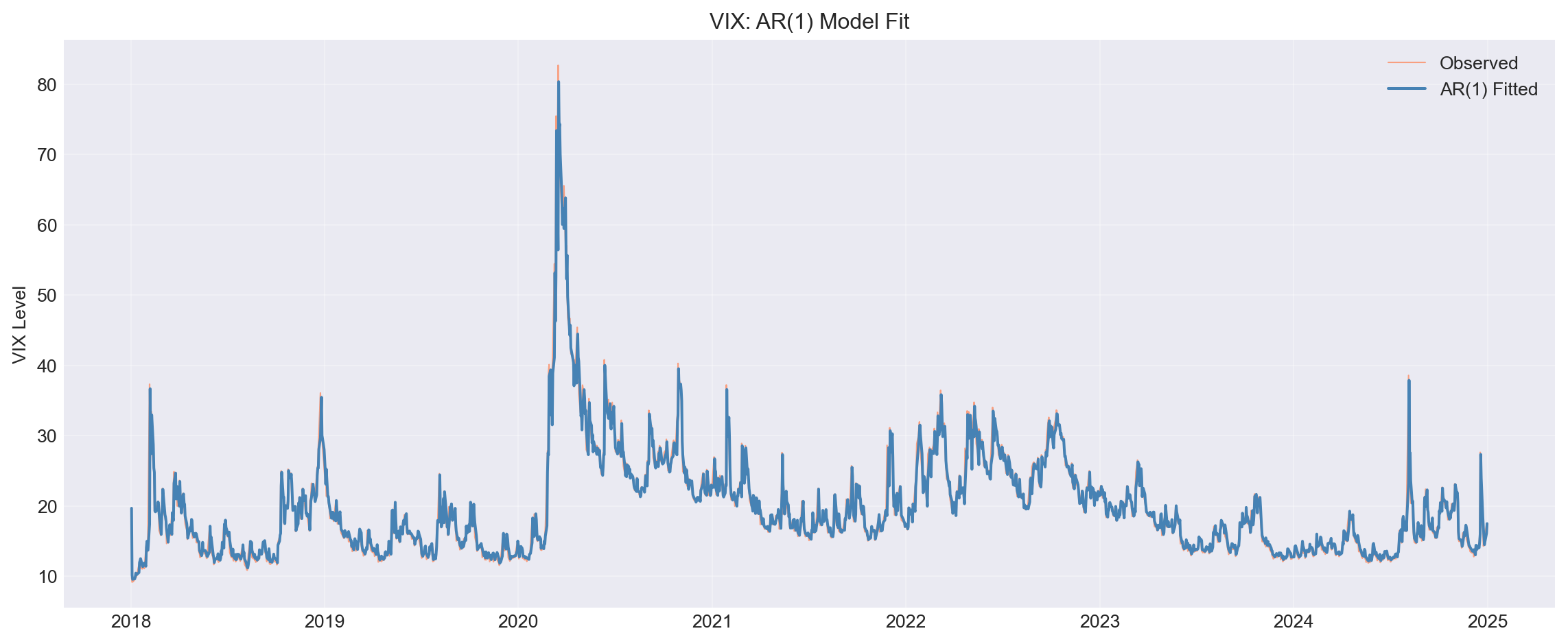
### 3.1 AR(1) Model for VIX
Let's fit an AR(1) model: $VIX_t = c + \phi_1 VIX_{t-1} + \varepsilon_t$
```{python}
#| label: ar1-fit
# Fit AR(1) = ARIMA(1,0,0)
model_ar1 = ARIMA(vix['PX_LAST'].dropna(), order=(1, 0, 0))
results_ar1 = model_ar1.fit()

# Print summary
print(results_ar1.summary())

# Plot fitted values
fig, ax = plt.subplots(figsize=(12, 5))
ax.plot(vix.index, vix['PX_LAST'], label='Observed',
        linewidth=0.8, alpha=0.7, color='coral')
ax.plot(vix.index, results_ar1.fittedvalues,
        label='AR(1) Fitted', linewidth=1.5, color='steelblue')
ax.set_ylabel('VIX Level')
ax.set_title('VIX: AR(1) Model Fit')
ax.legend()
ax.grid(alpha=0.3)
plt.tight_layout()
plt.show()
```
::: {.callout-note}
## Question 3.1
- Is the AR coefficient ($\phi_1$) significantly different from zero?
- What is the value of $\phi_1$? How persistent is VIX?
- Does the fitted line track the observed VIX reasonably well?
:::
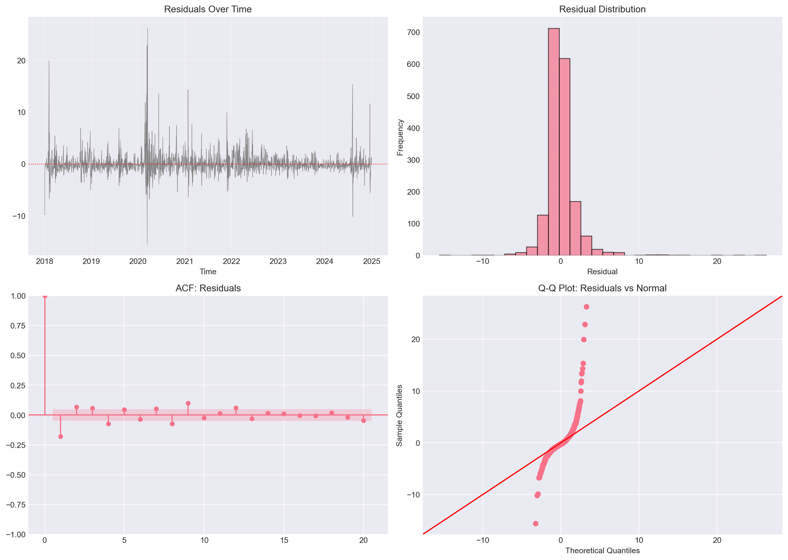
### 3.2 Model Diagnostics: Residuals
Good models should have **white noise residuals** (uncorrelated, mean zero). The **Ljung–Box test** jointly tests whether the first $m$ autocorrelations of the residuals are zero: $H_0$: $\rho_1 = \cdots = \rho_m = 0$. If the p-value is **greater than 0.05**, we fail to reject $H_0$ and treat residuals as white noise; if p-value **less than 0.05**, we reject and should consider more lags or a different model (Tsay, 2010, Ch 2).
```{python}
#| label: ar1-diagnostics
# Get residuals
residuals = results_ar1.resid

fig, axes = plt.subplots(2, 2, figsize=(14, 10))

# Time plot
axes[0, 0].plot(residuals, linewidth=0.5, color='gray')
axes[0, 0].axhline(0, color='red', linestyle='--', linewidth=0.5)
axes[0, 0].set_title('Residuals Over Time')
axes[0, 0].set_xlabel('Time')
axes[0, 0].grid(alpha=0.3)

# Histogram
axes[0, 1].hist(residuals, bins=30, edgecolor='black', alpha=0.7)
axes[0, 1].set_title('Residual Distribution')
axes[0, 1].set_xlabel('Residual')
axes[0, 1].set_ylabel('Frequency')
axes[0, 1].grid(alpha=0.3)

# ACF
plot_acf(residuals, ax=axes[1, 0], lags=20, title='ACF: Residuals')

# Q-Q plot
sm.qqplot(residuals, line='45', ax=axes[1, 1])
axes[1, 1].set_title('Q-Q Plot: Residuals vs Normal')

plt.tight_layout()
plt.show()

# Ljung-Box test for residual autocorrelation
from statsmodels.stats.diagnostic import acorr_ljungbox
lb_test = acorr_ljungbox(residuals, lags=10, return_df=True)
print("\nLjung-Box Test (H0: residuals are white noise):")
print(lb_test[['lb_stat', 'lb_pvalue']].head())
```
::: {.callout-note}
## Question 3.2
- Do residuals look randomly scattered around zero?
- Is there remaining autocorrelation in the ACF plot?
- Are residuals approximately normally distributed?
:::
### 3.3 Exercise: Fit ARIMA to SPY Prices
**Your task:** SPY prices are non-stationary. Fit an ARIMA(1,1,0) model (random walk with drift).
```{python}
#| label: spy-arima-exercise
# YOUR CODE HERE:
# 1. Fit ARIMA(1,1,0) to SPY prices
# 2. Print summary
# 3. Plot fitted values
# 4. Check residuals

# Solution (uncomment to run):
# model_spy = ARIMA(spy['PX_LAST'].dropna(), order=(1, 1, 0))
# results_spy = model_spy.fit()
# print(results_spy.summary())
#
# fig, ax = plt.subplots(figsize=(12, 5))
# ax.plot(spy.index, spy['PX_LAST'], label='Observed', alpha=0.7)
# ax.plot(spy.index, results_spy.fittedvalues, label='ARIMA(1,1,0) Fitted')
# ax.legend()
# plt.show()
```
::: {.callout-tip}
## Hint
ARIMA(1,1,0) = first difference + AR(1) = random walk with mean-reversion tendency.
:::
## Part 4: Forecasting and Validation
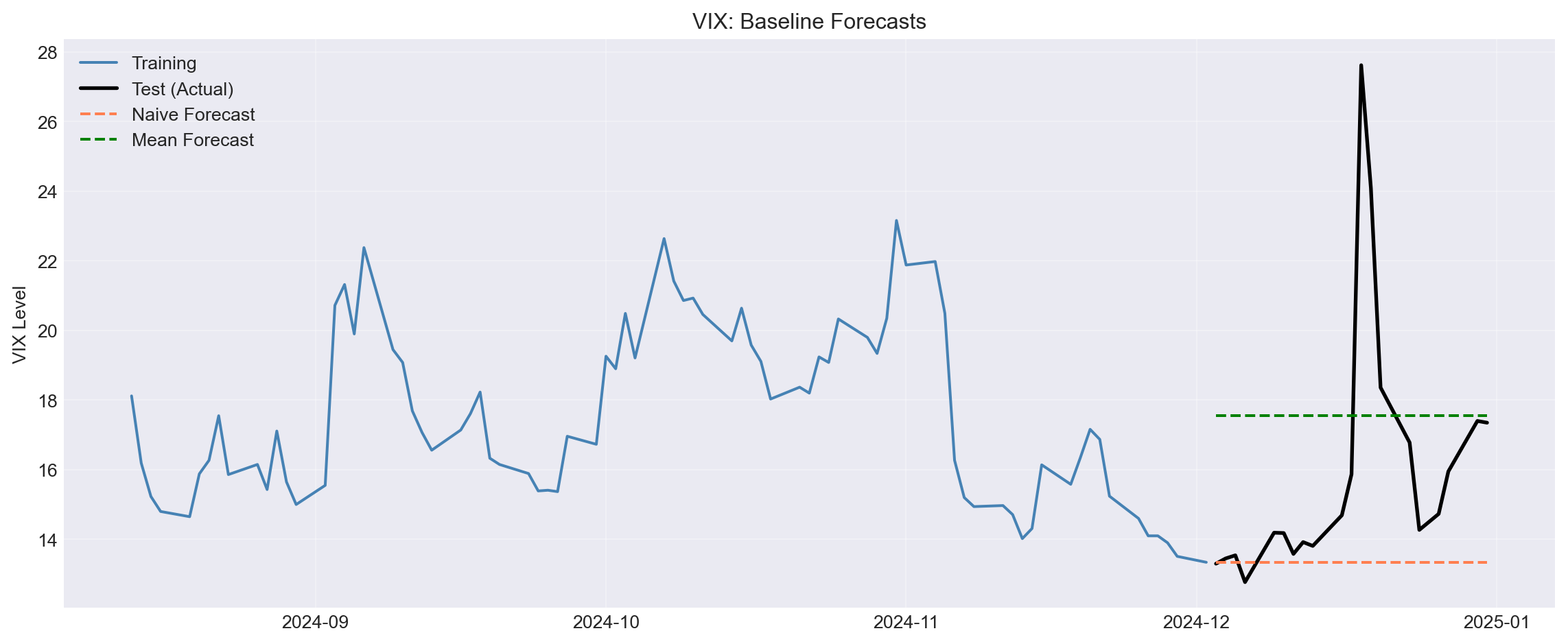
### 4.1 Simple Baselines
Before fitting complex models, establish **naive** and **mean** baselines.
```{python}
#| label: baselines
# Use last 100 days for demonstration
vix_recent = vix['PX_LAST'].iloc[-100:].dropna()

# Split: 80% train, 20% test
train_size = int(0.8 * len(vix_recent))
vix_train = vix_recent.iloc[:train_size]
vix_test = vix_recent.iloc[train_size:]

# Naive forecast: last observed value
naive_pred = np.full_like(vix_test, vix_train.iloc[-1])

# Mean forecast: historical average
mean_pred = np.full_like(vix_test, vix_train.mean())

# Plot
fig, ax = plt.subplots(figsize=(12, 5))
ax.plot(vix_train.index, vix_train, label='Training', color='steelblue')
ax.plot(vix_test.index, vix_test, label='Test (Actual)',
        color='black', linewidth=2)
ax.plot(vix_test.index, naive_pred, label='Naive Forecast',
        linestyle='--', color='coral')
ax.plot(vix_test.index, mean_pred, label='Mean Forecast',
        linestyle='--', color='green')
ax.set_ylabel('VIX Level')
ax.set_title('VIX: Baseline Forecasts')
ax.legend()
ax.grid(alpha=0.3)
plt.tight_layout()
plt.show()

# Accuracy
naive_mae = mean_absolute_error(vix_test, naive_pred)
mean_mae = mean_absolute_error(vix_test, mean_pred)

print(f"Naive MAE: {naive_mae:.4f}")
print(f"Mean MAE: {mean_mae:.4f}")
print(f"\nBest baseline: {'Naive' if naive_mae < mean_mae else 'Mean'}")
```
::: {.callout-note}
## Question 4.1
- Which baseline performs better?
- Why might the mean forecast work well for VIX?
:::
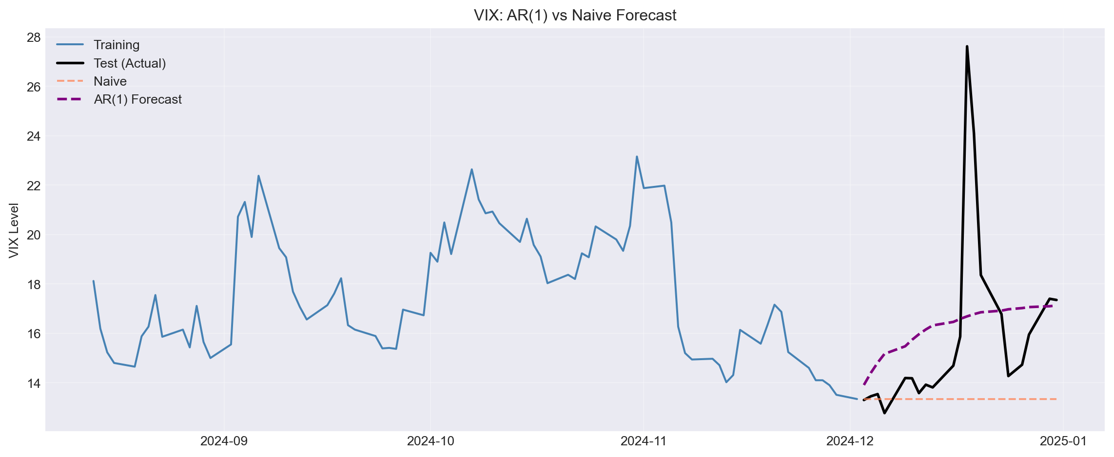
### 4.2 AR(1) vs Baselines
Does AR(1) beat naive?
```{python}
#| label: ar1-forecast
# Fit AR(1) on training data
model_train = ARIMA(vix_train, order=(1, 0, 0))
results_train = model_train.fit()

# Forecast
forecast = results_train.forecast(steps=len(vix_test))

# Plot
fig, ax = plt.subplots(figsize=(12, 5))
ax.plot(vix_train.index, vix_train, label='Training', color='steelblue')
ax.plot(vix_test.index, vix_test, label='Test (Actual)',
        color='black', linewidth=2)
ax.plot(vix_test.index, naive_pred, label='Naive',
        linestyle='--', color='coral', alpha=0.7)
ax.plot(vix_test.index, forecast.values, label='AR(1) Forecast',
        linestyle='--', color='purple', linewidth=2)
ax.set_ylabel('VIX Level')
ax.set_title('VIX: AR(1) vs Naive Forecast')
ax.legend()
ax.grid(alpha=0.3)
plt.tight_layout()
plt.show()

# Accuracy
ar1_mae = mean_absolute_error(vix_test, forecast)

print(f"\nForecast Accuracy (MAE):")
print(f"  Naive:  {naive_mae:.4f}")
print(f"  Mean:   {mean_mae:.4f}")
print(f"  AR(1):  {ar1_mae:.4f}")
print(f"\nBest model: AR(1)" if ar1_mae < min(naive_mae, mean_mae) else "Best model: Baseline")
```
::: {.callout-note}
## Question 4.2
- Does AR(1) beat the baselines?
- If yes, by how much?
- Is the improvement economically meaningful?
:::
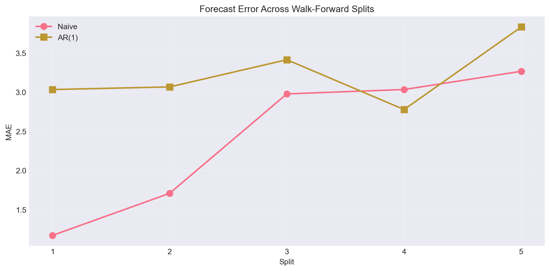
### 4.3 Walk-Forward Validation
Single train/test split is risky. Use **time series cross-validation**.
```{python}
#| label: walk-forward
# Use full VIX series
vix_full = vix['PX_LAST'].dropna()

# Walk-forward with 5 splits
tscv = TimeSeriesSplit(n_splits=5, test_size=50)

naive_errors = []
ar1_errors = []

for train_idx, test_idx in tscv.split(vix_full):
    # Split
    train = vix_full.iloc[train_idx]
    test = vix_full.iloc[test_idx]

    # Naive forecast
    naive_pred = np.full_like(test, train.iloc[-1])
    naive_errors.append(mean_absolute_error(test, naive_pred))

    # AR(1) forecast
    model = ARIMA(train, order=(1, 0, 0))
    results = model.fit()
    ar1_pred = results.forecast(steps=len(test))
    ar1_errors.append(mean_absolute_error(test, ar1_pred))

# Results
print("Walk-Forward Cross-Validation (5 splits):")
print(f"  Naive MAE (average): {np.mean(naive_errors):.4f} ± {np.std(naive_errors):.4f}")
print(f"  AR(1) MAE (average): {np.mean(ar1_errors):.4f} ± {np.std(ar1_errors):.4f}")
print(f"\nWinner: {'AR(1)' if np.mean(ar1_errors) < np.mean(naive_errors) else 'Naive'}")

# Plot errors across splits
fig, ax = plt.subplots(figsize=(10, 5))
x = np.arange(1, 6)
ax.plot(x, naive_errors, 'o-', label='Naive', linewidth=2, markersize=8)
ax.plot(x, ar1_errors, 's-', label='AR(1)', linewidth=2, markersize=8)
ax.set_xlabel('Split')
ax.set_ylabel('MAE')
ax.set_title('Forecast Error Across Walk-Forward Splits')
ax.set_xticks(x)
ax.legend()
ax.grid(alpha=0.3)
plt.tight_layout()
plt.show()
```
::: {.callout-note}
## Question 4.3
- Is AR(1) consistently better than naive across all splits?
- What does the variability across splits tell you?
:::
### 4.4 The ARIMA Reality Check: Returns vs Levels
The previous exercises used VIX *levels*, which are mean-reverting (AR(1) has signal). But what about **returns**? This is the crucial test of whether ARIMA adds value for the problem most practitioners care about.
```{python}
#| label: arima-reality-check
# SPY returns (not prices, not VIX)
spy_returns = spy['return'].dropna()

# Walk-forward CV for returns
tscv = TimeSeriesSplit(n_splits=5, test_size=50)

naive_ret_errors = []
ar1_ret_errors = []
zero_ret_errors = []  # Predicting zero (simplest naive for returns)

for train_idx, test_idx in tscv.split(spy_returns):
    train = spy_returns.iloc[train_idx]
    test = spy_returns.iloc[test_idx]

    # Naive: predict last return
    naive_pred = np.full_like(test, train.iloc[-1])
    naive_ret_errors.append(mean_absolute_error(test, naive_pred))

    # Zero forecast (returns fluctuate around zero)
    zero_pred = np.zeros_like(test)
    zero_ret_errors.append(mean_absolute_error(test, zero_pred))

    # AR(1) for returns
    try:
        model = ARIMA(train, order=(1, 0, 0))
        results = model.fit()
        ar1_pred = results.forecast(steps=len(test))
        ar1_ret_errors.append(mean_absolute_error(test, ar1_pred))
    except:
        ar1_ret_errors.append(np.nan)

# Results
print("=== THE ARIMA REALITY CHECK ===")
print("\nPredicting SPY Daily RETURNS (not VIX levels):")
print(f"  Zero forecast MAE: {np.mean(zero_ret_errors):.6f}")
print(f"  Naive forecast MAE: {np.mean(naive_ret_errors):.6f}")
print(f"  AR(1) forecast MAE: {np.nanmean(ar1_ret_errors):.6f}")

# Compare to zero
ar1_improvement = (np.mean(zero_ret_errors) - np.nanmean(ar1_ret_errors)) / np.mean(zero_ret_errors) * 100
print(f"\nAR(1) improvement over zero: {ar1_improvement:.2f}%")

if ar1_improvement < 1:
    print("\n⚠️ KEY INSIGHT: AR(1) barely beats predicting zero!")
    print("   For returns, the mean equation is almost trivial.")
    print("   This is why we focus on VOLATILITY modelling (Week 4).")
```
::: {.callout-important}
## The Three Prediction Problems
This exercise demonstrates a fundamental insight:
| What You Predict | Signal? | Does ARIMA Help? |
|------------------|---------|------------------|
| VIX levels (mean-reverting) | Yes (~25% R²) | ✓ AR(1) beats naive |
| SPY returns | Almost none (~1% R²) | ✗ Barely beats zero |
| Volatility (squared returns) | Yes | ✓ GARCH family (Week 4) |
**The lesson:** Don't waste time fitting complex ARIMA models to returns. The signal is in the *variance* (volatility), not the *mean* (returns). This is why GARCH matters.
**Connection to signal-to-noise:** For an AR(1) model, R² = ρ² (squared first-order autocorrelation). So autocorrelation directly measures predictability: where autocorrelation is strong (VIX, squared returns), signal exists; where it's weak (returns), noise dominates. This connects directly to the signal vs noise framing on the [course homepage](../index.qmd#acting-in-the-dark): returns have R² < 5% because they're approximately white noise. The Three Prediction Problems hierarchy reflects where autocorrelation: and therefore predictable signal: actually lives.
:::
::: {.callout-note}
## Question 4.4
1. How much did AR(1) improve over simply predicting zero?
2. Is this improvement economically meaningful after transaction costs?
3. Why does AR(1) work for VIX levels but not SPY returns?
:::
## Part 5: Challenge Exercises
### 5.1 Exercise: BTCUSD (Highly Non-Stationary)
Bitcoin is highly volatile and non-stationary. Test different ARIMA specifications.
```{python}
#| label: btc-challenge
# Extract BTCUSD
btc = df[df['ticker'] == 'BTCUSD'].set_index('date').sort_index()

# YOUR TASK:
# 1. Test stationarity of BTC prices and returns
# 2. Fit ARIMA(0,1,0) (random walk) to prices
# 3. Compare to naive forecast
# 4. Does ARIMA add value?
```
### 5.2 Exercise: Treasury Yield (Mean-Reverting?)
The 10-year Treasury yield may be mean-reverting or trending depending on the period.
```{python}
#| label: treasury-challenge
# Extract USGG10YR
treasury = df[df['ticker'] == 'USGG10YR'].set_index('date').sort_index()

# YOUR TASK:
# 1. Visual and statistical stationarity tests
# 2. Fit AR(1) or ARIMA(1,1,0) depending on stationarity
# 3. Forecast and evaluate
```
## Summary
In this lab, you learned to:
1. ✓ Diagnose stationarity using visual and ADF tests
2. ✓ Interpret ACF/PACF to identify AR vs MA patterns
3. ✓ Fit and diagnose ARIMA models
4. ✓ Perform walk-forward validation
5. ✓ Compare forecasts to naive baselines
**Key takeaways:**
- Prices are non-stationary; returns are (mostly) stationary
- VIX is mean-reverting but persistent → AR(1) fits well
- Always compare to naive forecast : if you can't beat it, use it
- Walk-forward validation prevents overfitting
## References
- Tsay, R. S. (2010). *Analysis of Financial Time Series*, 3rd ed. Wiley. Chapter 2 (Linear Time Series), Chapter 3 (Conditional Heteroscedastic Models).
- Brooks, C. (2019). *Introductory Econometrics for Finance*, 4th ed. Cambridge University Press. Chapter 5 (Univariate time series modelling and forecasting).
- Hyndman, R. J., & Athanasopoulos, G. (2021). *Forecasting: Principles and Practice*, 3rd ed.