Lab 03: SPY and VIX Time Series Extraction

In-Class Bloomberg Terminal Session : Week 3

ImportantIn-Class Lab Structure

This is the in-class Bloomberg lab for Week 3, conducted in the Financial Innovation Lab.

Before class: Complete the homework (Lab 3: Time Series Foundations) in Colab to learn stationarity, ACF/PACF, and ARIMA. The homework uses pre-collected Bloomberg data from our shared database.

In class: Extract SPY and VIX yourself from the Bloomberg Terminal. Export to CSV, then run stationarity diagnostics on your own data. This levels your Terminal access with Week 2 and reinforces where the data comes from.

Open in Colab

Lab Overview

Type: In-class lab (Bloomberg Terminal, supervised)

Duration: 45–60 minutes

Location: Financial Innovation Lab (~20 Bloomberg terminals)

Learning Objectives:

1. Extract historical time series (SPY, VIX) from Bloomberg using BDH
2. Export to CSV for Python analysis
3. Run stationarity diagnostics on your own extraction
4. Connect the in-class extraction to the homework lab (Colab)

Prerequisites:

• Complete Lab 3 homework (time series foundations) : you’ll recognise the analysis
• Bring laptop for Python (Colab or local) : Bloomberg extraction on terminals

Background

Lab 3 (homework) uses SPY and VIX from our pre-collected Bloomberg database. Here you extract the same series yourself. SPY tracks the S&P 500; VIX measures implied volatility. Both are central to time series diagnostics: SPY returns are hard to predict; VIX levels are mean-reverting.

Part 1: Bloomberg Data Extraction (25–30 minutes)

Step 1: Bloomberg Setup

1. Log in to the Bloomberg Terminal
2. Open Excel then close it again
3. Install the Bloomberg Excel Add-in (right-hand side of home screen : required each session)
4. Open Excel and begin extraction

Step 2: Extract SPY

Use the BDH (Bloomberg Data History) function.

In Excel:

Cell A1: =BDH("SPY US Equity", "PX_LAST", "20190101", "20241231", "Days", "A")

This retrieves daily closing prices for SPY from 1 Jan 2019 to 31 Dec 2024.

Step 3: Extract VIX

Cell C1: =BDH("VIX Index", "PX_LAST", "20190101", "20241231", "Days", "A")

Step 4: Save to CSV

1. Ensure columns: Date, SPY (or “SPY US Equity”), VIX (or “VIX Index”)
2. Save as CSV: spy_vix_2019_2024.csv
3. You’ll upload this in Part 2

TipColumn Names

Bloomberg may use “SPY US Equity” and “VIX Index”. The code below normalises these to SPY and VIX.

Part 2: Stationarity Diagnostics (25–30 minutes)

Upload your CSV in Colab (or load locally) and run the same diagnostics as the homework lab.

import pandas as pd
import numpy as np
from pathlib import Path

# Colab: prompt for upload
IN_COLAB = False
try:
    import google.colab
    IN_COLAB = True
except ImportError:
    pass

uploaded_path = None
if IN_COLAB:
    from google.colab import files
    uploaded = files.upload()
    if uploaded:
        uploaded_path = list(uploaded.keys())[0]
        print(f"Uploaded: {uploaded_path}")
else:
    for name in ["spy_vix_2019_2024.csv", "spy_vix_data.csv"]:
        if Path(name).exists():
            uploaded_path = name
            print(f"Using local file: {uploaded_path}")
            break

if uploaded_path is None:
    print("No CSV found. Load from shared database instead.")

No CSV found. Load from shared database instead.

import matplotlib.pyplot as plt
from statsmodels.tsa.stattools import adfuller
from statsmodels.graphics.tsaplots import plot_acf

# Load your CSV or fallback to parquet
if 'uploaded_path' in dir() and uploaded_path is not None:
    df = pd.read_csv(uploaded_path)
    df.columns = df.columns.str.strip()
    date_col = 'Date' if 'Date' in df.columns else df.columns[0]
    df[date_col] = pd.to_datetime(df[date_col])
    df = df.set_index(date_col).sort_index()
    # Normalise column names (Bloomberg may use "SPY US Equity", "VIX Index")
    renames = {}
    for c in df.columns:
        if c == date_col:
            continue
        if 'SPY' in str(c).upper():
            renames[c] = 'SPY'
        elif 'VIX' in str(c).upper():
            renames[c] = 'VIX'
    df = df.rename(columns=renames)
    print("Loaded your Bloomberg extraction.")
else:
    # Fallback: shared parquet
    url = "https://raw.githubusercontent.com/quinfer/fin510-colab-notebooks/main/resources/bloomberg_database.parquet"
    full = pd.read_parquet(url)
    spy = full[full['ticker'] == 'SPY'][['date', 'PX_LAST']].rename(columns={'date': 'Date', 'PX_LAST': 'SPY'}).set_index('Date')
    vix = full[full['ticker'] == 'VIX'][['date', 'PX_LAST']].rename(columns={'date': 'Date', 'PX_LAST': 'VIX'}).set_index('Date')
    df = spy.join(vix, how='inner')
    df = df.loc['2019':'2024']
    print("Using shared database (no CSV uploaded).")

# Prepare series
spy_prices = df['SPY'].dropna()
spy_returns = spy_prices.pct_change().dropna()
vix_levels = df['VIX'].dropna()

# ADF tests
def adf_report(series, name):
    result = adfuller(series.dropna())
    print(f"{name}: ADF stat = {result[0]:.4f}, p-value = {result[1]:.4f}")
    print(f"  → {'Stationary' if result[1] < 0.05 else 'Non-stationary'} at 5%")

print("\n--- Stationarity (ADF Test) ---")
adf_report(spy_prices, "SPY Prices")
adf_report(spy_returns, "SPY Returns")
adf_report(vix_levels, "VIX Levels")

# Quick plot
fig, axes = plt.subplots(2, 1, figsize=(12, 6), sharex=True)
axes[0].plot(spy_prices.index, spy_prices.values, linewidth=0.8, color='steelblue')
axes[0].set_ylabel('SPY Price')
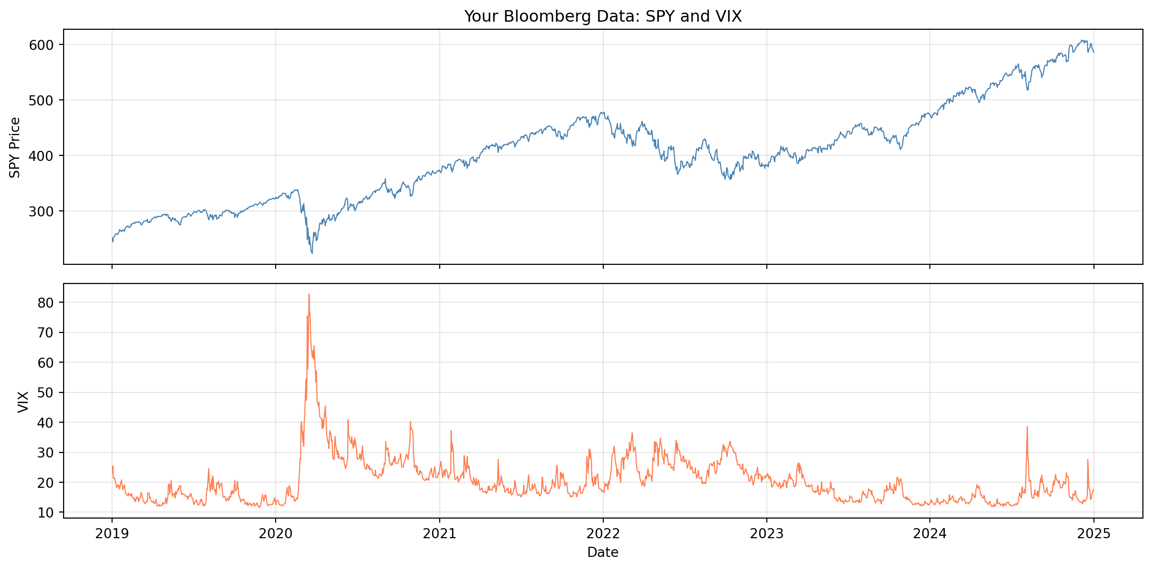
axes[0].set_title('Your Bloomberg Data: SPY and VIX')
axes[0].grid(alpha=0.3)
axes[1].plot(vix_levels.index, vix_levels.values, linewidth=0.8, color='coral')
axes[1].set_ylabel('VIX')
axes[1].set_xlabel('Date')
axes[1].grid(alpha=0.3)
plt.tight_layout()
plt.show()

Using shared database (no CSV uploaded).

--- Stationarity (ADF Test) ---
SPY Prices: ADF stat = -0.4809, p-value = 0.8957
  → Non-stationary at 5%
SPY Returns: ADF stat = -11.6514, p-value = 0.0000
  → Stationary at 5%
VIX Levels: ADF stat = -4.3206, p-value = 0.0004
  → Stationary at 5%

NoteCompare with Homework

Does your extraction match the homework lab’s conclusions? SPY prices non-stationary, returns borderline; VIX mean-reverting. If your date range differs, results may vary slightly.

Complete the rest at home: The full diagnostic suite (ACF, PACF, volatility clustering, ARIMA fitting, and the Three Prediction Problems comparison) is in the homework lab. Work through Lab 3: Time Series Foundations in Colab to complete the analysis.

TipConnecting to Signal-to-Noise

The autocorrelation differences you observe connect directly to the Three Prediction Problems on the course homepage:

• SPY returns: Weak autocorrelation → low signal-to-noise → ~1% R² → hard to predict
• VIX levels: Strong autocorrelation → higher signal-to-noise → ~25% R² → AR(1) works

For an AR(1) model, R² = ρ² (squared autocorrelation). So autocorrelation directly measures predictability. Where autocorrelation is weak (returns), noise dominates. Where it’s strong (VIX, volatility), signal exists. This is why we focus on volatility modelling (Week 4) rather than trying to forecast returns.

Summary

You extracted SPY and VIX from Bloomberg, exported to CSV, and ran ADF stationarity diagnostics. Complete the full diagnostic suite at home (ACF, PACF, ARIMA, Three Prediction Problems) using the homework lab: open it in Colab from the course website. Next week (Lab 4) we use Bloomberg for volatility (VIX vs realised volatility).