Show code
try:
    import numpy
    import matplotlib
    import scipy
except Exception:
!pip -q install numpy matplotlib scipyCost structures, portfolio optimisation, and welfare analysis
This lab includes interpretation questions asking you to write 150-500 words explaining your results. Attempt these independently first, then compare your answers to the sample responses provided in collapsible boxes throughout the HTML version of this lab on the course website.
The sample answers demonstrate the depth of analysis, evidence integration, and academic writing style expected in coursework assessments.
![]()
try:
import numpy
import matplotlib
import scipy
except Exception:
!pip -q install numpy matplotlib scipyBy the end of this lab, you will be able to:
This plan keeps you moving between economics, algorithms, and policy implications. You can extend with sensitivity analyses in directed learning.
Before we code, let’s understand the economic transformation. Traditional wealth managers charge percentage fees (e.g., 1.5% of assets under management) but impose minimum fees (e.g., $2,500/year) that make small accounts unprofitable. This creates exclusion: if you have $10,000 to invest, a $2,500 fee is 25% of your wealth: prohibitively expensive.
Robo-advisers eliminate fixed costs through automation. They charge lower percentage fees (e.g., 0.25%) with no minimums. The same $10,000 account costs $25/year: a 100x reduction. This cost structure change is why robo-advisers expand access to middle-class investors.
Our lab explores this economics quantitatively, then implements the algorithms that enable automation.
Let’s visualise how fees differ across account sizes and calculate the access implications.
import numpy as np
import matplotlib.pyplot as plt

# Define fee structures
account_sizes = np.array([10_000, 25_000, 50_000, 100_000, 250_000, 500_000, 1_000_000])

# Traditional adviser
trad_rate = 0.015  # 1.5% AUM
trad_min = 2500    # $2,500 minimum annual fee
trad_fee = np.maximum(account_sizes * trad_rate, trad_min)

# Robo-adviser
robo_rate = 0.0025  # 0.25% AUM
robo_min = 0        # No minimum
robo_fee = account_sizes * robo_rate + robo_min

# Calculate effective rates (actual fee as % of assets)
trad_effective = (trad_fee / account_sizes) * 100
robo_effective = (robo_fee / account_sizes) * 100

# Calculate savings
annual_savings = trad_fee - robo_fee
savings_pct = (annual_savings / trad_fee) * 100

# Visualization
fig, axes = plt.subplots(2, 2, figsize=(14, 10))

# Panel 1: Annual Fees (log scale)
axes[0, 0].plot(account_sizes/1000, trad_fee, 'o-', linewidth=2, markersize=8,
                label='Traditional Adviser', color='tab:blue')
axes[0, 0].plot(account_sizes/1000, robo_fee, 's-', linewidth=2, markersize=8,
                label='Robo-Adviser', color='tab:red')
axes[0, 0].set_xlabel('Account Size ($000s)', fontsize=11)
axes[0, 0].set_ylabel('Annual Fee ($)', fontsize=11)
axes[0, 0].set_title('Annual Advisory Fees by Account Size', fontsize=12, pad=10)
axes[0, 0].legend(fontsize=10)
axes[0, 0].grid(alpha=0.3, linestyle=':')
axes[0, 0].set_yscale('log')

# Panel 2: Effective Fee Rates
axes[0, 1].plot(account_sizes/1000, trad_effective, 'o-', linewidth=2, markersize=8,
                label='Traditional', color='tab:blue')
axes[0, 1].plot(account_sizes/1000, robo_effective, 's-', linewidth=2, markersize=8,
                label='Robo-Adviser', color='tab:red')
axes[0, 1].axhline(0.25, color='red', linestyle=':', alpha=0.5, label='Robo flat rate')
axes[0, 1].set_xlabel('Account Size ($000s)', fontsize=11)
axes[0, 1].set_ylabel('Effective Fee Rate (%)', fontsize=11)
axes[0, 1].set_title('Effective Fee Rates (Actual Fee / Assets)', fontsize=12, pad=10)
axes[0, 1].legend(fontsize=9)
axes[0, 1].grid(alpha=0.3, linestyle=':')

# Panel 3: Annual Savings
axes[1, 0].bar(range(len(account_sizes)), annual_savings, alpha=0.7, color='green')
axes[1, 0].set_xlabel('Account Size Category', fontsize=11)
axes[1, 0].set_ylabel('Annual Savings ($)', fontsize=11)
axes[1, 0].set_title('Annual Cost Savings with Robo-Adviser', fontsize=12, pad=10)
axes[1, 0].set_xticks(range(len(account_sizes)))
axes[1, 0].set_xticklabels([f'${s/1000:.0f}K' for s in account_sizes], rotation=45)
axes[1, 0].grid(alpha=0.3, axis='y', linestyle=':')

for i, v in enumerate(annual_savings):
    axes[1, 0].text(i, v + 100, f'${v:,.0f}', ha='center', va='bottom', fontsize=9)

# Panel 4: Compound Savings Over 20 Years
years = 20
return_rate = 0.06
compound_savings = []

for size, saving in zip(account_sizes, annual_savings):
    fv_savings = saving * ((1 + return_rate)**years - 1) / return_rate
    compound_savings.append(fv_savings)

axes[1, 1].bar(range(len(account_sizes)), np.array(compound_savings)/1000, alpha=0.7, color='purple')
axes[1, 1].set_xlabel('Account Size Category', fontsize=11)
axes[1, 1].set_ylabel('Compound Savings ($000s)', fontsize=11)
axes[1, 1].set_title(f'20-Year Compound Savings (6% return)', fontsize=12, pad=10)
axes[1, 1].set_xticks(range(len(account_sizes)))
axes[1, 1].set_xticklabels([f'${s/1000:.0f}K' for s in account_sizes], rotation=45)
axes[1, 1].grid(alpha=0.3, axis='y', linestyle=':')

plt.suptitle('Traditional vs. Robo-Adviser Fee Analysis', fontsize=14, y=0.995)
plt.tight_layout()
plt.show()

# Validation
assert trad_fee[0] == trad_min, "Minimum fee should apply to smallest account"
assert np.allclose(robo_effective, robo_rate * 100), "Robo effective rate should be constant"
assert all(annual_savings > 0), "Robo should always be cheaper"

print("✔ Fee calculation validation passed\n")
print("Summary Statistics:")
print("=" * 60)
print(f"{'Account':<12} {'Trad Fee':<12} {'Robo Fee':<12} {'Savings':<12} {'Compound 20Y':<12}")
print("-" * 60)
for i, size in enumerate(account_sizes):
    print(f"${size:<11,} ${trad_fee[i]:<11,.0f} ${robo_fee[i]:<11,.0f} "
          f"${annual_savings[i]:<11,.0f} ${compound_savings[i]:<11,.0f}")

break_even = trad_min / trad_rate
print(f"\n✔ Traditional adviser break-even account size: ${break_even:,.0f}")
print(f"   (Below this, effective rate exceeds {trad_rate*100:.1f}% due to minimum fee)")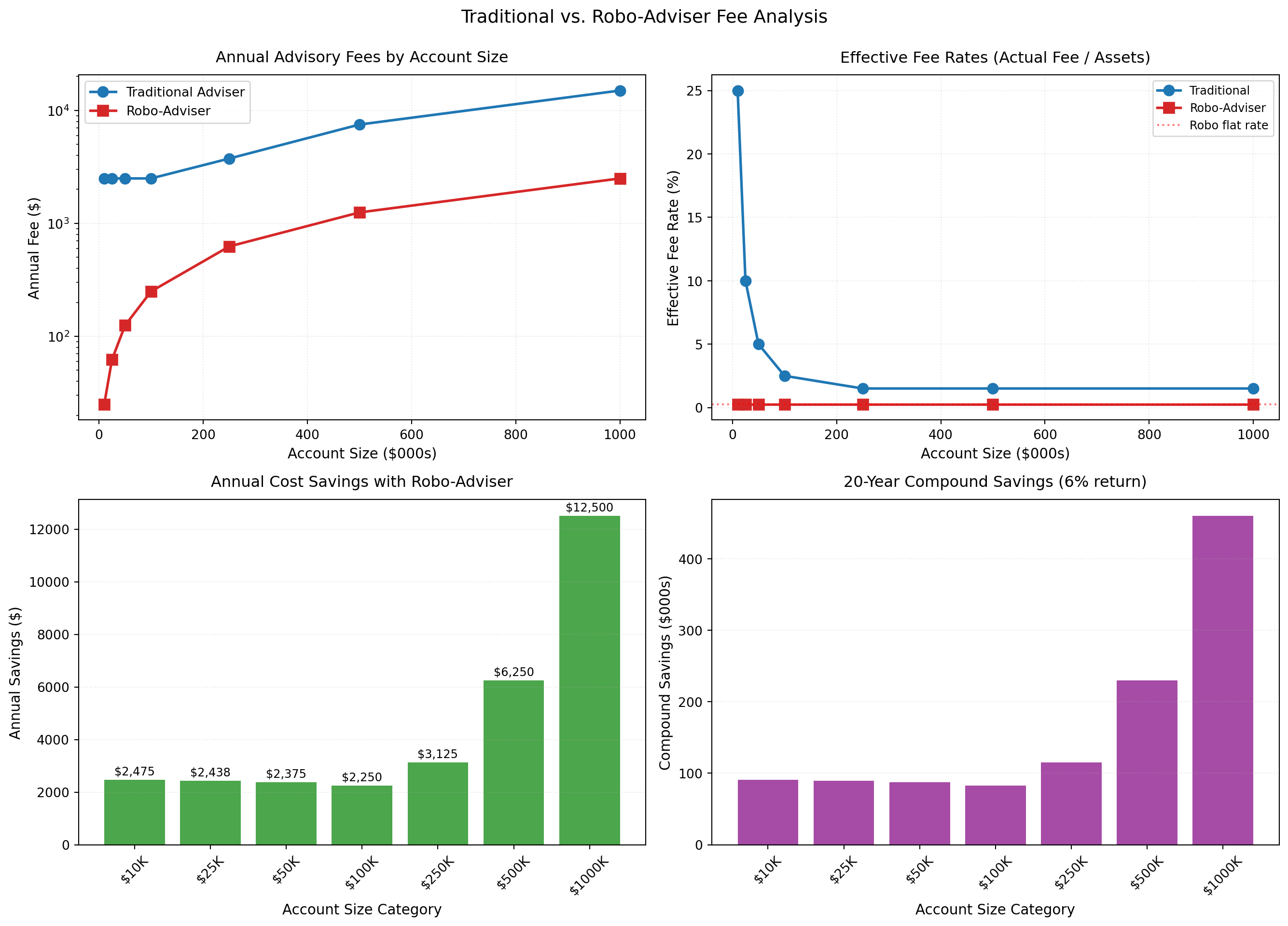
✔ Fee calculation validation passed

Summary Statistics:
============================================================
Account      Trad Fee     Robo Fee     Savings      Compound 20Y
------------------------------------------------------------
$10,000      $2,500       $25          $2,475       $91,044
$25,000      $2,500       $62          $2,438       $89,665
$50,000      $2,500       $125         $2,375       $87,366
$100,000     $2,500       $250         $2,250       $82,768
$250,000     $3,750       $625         $3,125       $114,955
$500,000     $7,500       $1,250       $6,250       $229,910
$1,000,000   $15,000      $2,500       $12,500      $459,820

✔ Traditional adviser break-even account size: $166,667
(Below this, effective rate exceeds 1.5% due to minimum fee)Study the four panels and answer:
Effective rate panel (top right): Notice the traditional effective rate is 25% for a $10K account. Why does this make traditional advice economically infeasible for small investors?
Access barrier: At what account size does traditional advice become “affordable” (effective rate drops below 2%)? How many households does this exclude?
Compound savings panel (bottom right): A $100K account saves $1,250/year. Over 20 years at 6% returns, this becomes ~$48K. What does this tell you about the lifetime wealth impact of fee compression?
Break-even calculation: What happens to traditional advisers’ business models as robo-advisers capture accounts below this threshold?
Write 200–300 words interpreting these results and connecting to Reher and Sokolinski (2024)’s evidence on access expansion and welfare gains.
The visualisations reveal the fundamental economic barrier that traditional wealth management creates for small investors. The effective rate panel demonstrates this starkly: at a £10,000 account size, the traditional model charges an effective rate of 25%, making professional advice economically irrational. This isn’t merely expensive: it’s prohibitive. The minimum fee creates a hard exclusion boundary that no amount of cost-consciousness can overcome if you lack sufficient wealth.
The break-even analysis shows traditional advice becomes “affordable” (under 2% effective rate) only above £125,000 in assets. According to household wealth data, this excludes roughly 85-90% of UK households from accessing professional portfolio management. This aligns with Reher and Sokolinski’s (2024) finding that welfare gains from robo-advisers concentrate in the £25,000-£150,000 wealth range: precisely the segment excluded by traditional minimums but able to benefit from automated advice.
The compound savings panel illustrates why fee compression matters profoundly over investment horizons. A £100,000 account saves £1,250 annually, but compounded at 6% over 20 years, this becomes approximately £48,000: nearly half the initial investment. This demonstrates that fees aren’t just a cost; they’re a return drag that compounds negatively over time, eroding wealth systematically.
However, Reher and Sokolinski estimate welfare gains of only 0.3-0.7% of investable wealth, far smaller than naive fee savings suggest. Why? First, many investors in this wealth range were already investing through low-cost mutual funds or ETFs: robo-advisers improve but don’t create market access. Second, behavioural frictions limit take-up; not everyone excluded by traditional minimums adopts robo-advisers. Third, robo-adviser fees, whilst lower, aren’t zero. The welfare gain represents the net benefit after accounting for remaining costs and alternative options, not the gross fee difference. This nuance matters for evaluating democratisation claims: robo-advisers expand access meaningfully but modestly, not revolutionarily.
Now let’s implement the core algorithm robo-advisers use: Modern Portfolio Theory optimisation. We’ll find the portfolio that maximises the Sharpe ratio (risk-adjusted return).
import numpy as np
from scipy.optimize import minimize

class SimpleRoboAdvisor:
    """
    Minimal robo-advisor portfolio optimizer implementing Modern Portfolio Theory.

    This class demonstrates the core algorithm that robo-advisors use to construct
    optimal portfolios. Real platforms extend this with factor models, ESG constraints,
    tax-loss harvesting, and automatic rebalancing.

    Attributes
    ----------
    asset_names : list of str
        Names of assets in the investment universe
    expected_returns : ndarray
        Expected annual returns for each asset
    cov_matrix : ndarray
        Covariance matrix of annual returns (n_assets × n_assets)
    risk_free_rate : float
        Annual risk-free rate for Sharpe ratio calculation
    n_assets : int
        Number of assets in the universe

    Examples
    --------
    >>> assets = ['US Stocks', 'Bonds', 'Real Estate']
    >>> returns = np.array([0.10, 0.05, 0.08])
    >>> cov = np.array([[0.04, 0.01, 0.02],
    ...                 [0.01, 0.01, 0.005],
    ...                 [0.02, 0.005, 0.03]])
    >>> robo = SimpleRoboAdvisor(assets, returns, cov, risk_free_rate=0.02)
    >>> result = robo.optimize(max_position_size=0.50)
    >>> result['sharpe']  # Sharpe ratio of optimal portfolio
    1.45
    """

    def __init__(self, asset_names, expected_returns, cov_matrix, risk_free_rate=0.02):
        """
        Initialize robo-advisor with asset universe and market expectations.

        Parameters
        ----------
        asset_names : list of str
            Names of assets (e.g., ['US Stocks', 'Bonds', 'Real Estate'])
        expected_returns : array-like
            Expected annual returns for each asset (as decimals, e.g., 0.10 = 10%)
        cov_matrix : array-like
            Covariance matrix of annual returns (n_assets × n_assets)
        risk_free_rate : float, default=0.02
            Annual risk-free rate for Sharpe ratio calculation (as decimal)

        Raises
        ------
        AssertionError
            If dimensions of expected_returns or cov_matrix don't match asset_names
        """
        self.asset_names = asset_names
        self.expected_returns = np.array(expected_returns)
        self.cov_matrix = np.array(cov_matrix)
        self.risk_free_rate = risk_free_rate
        self.n_assets = len(asset_names)

        # Validate inputs
        assert len(self.expected_returns) == self.n_assets, \
            f"Expected {self.n_assets} returns, got {len(self.expected_returns)}"
        assert self.cov_matrix.shape == (self.n_assets, self.n_assets), \
            f"Covariance matrix should be {self.n_assets}×{self.n_assets}"

    def portfolio_return(self, weights):
        """
        Calculate expected portfolio return.

        Parameters
        ----------
        weights : array-like
            Asset weights (must sum to 1.0)

        Returns
        -------
        float
            Expected annual portfolio return
        """
        return np.dot(weights, self.expected_returns)

    def portfolio_volatility(self, weights):
        """
        Calculate portfolio volatility (standard deviation).

        Parameters
        ----------
        weights : array-like
            Asset weights (must sum to 1.0)

        Returns
        -------
        float
            Annual portfolio volatility (standard deviation)
        """
        return np.sqrt(np.dot(weights.T, np.dot(self.cov_matrix, weights)))

    def sharpe_ratio(self, weights):
        """
        Calculate Sharpe ratio (risk-adjusted return).

        Parameters
        ----------
        weights : array-like
            Asset weights (must sum to 1.0)

        Returns
        -------
        float
            Sharpe ratio = (portfolio_return - risk_free_rate) / portfolio_volatility
            Returns -inf if volatility is zero
        """
        ret = self.portfolio_return(weights)
        vol = self.portfolio_volatility(weights)
        if vol == 0:
            return -np.inf
        return (ret - self.risk_free_rate) / vol

    def optimize(self, max_position_size=0.50, allow_short=False):
        """
        Find the portfolio with maximum Sharpe ratio.

        This is the core optimization that robo-advisors perform: given expected
        returns and risk (covariance matrix), find the portfolio weights that
        maximize risk-adjusted returns subject to diversification constraints.

        Parameters
        ----------
        max_position_size : float, default=0.50
            Maximum weight in any single asset (e.g., 0.50 = max 50% in one asset).
            Enforces diversification.
        allow_short : bool, default=False
            Whether to allow short positions (negative weights).
            If False, all weights must be ≥ 0.

        Returns
        -------
        dict
            Optimal portfolio with keys:
            - 'weights' : ndarray, optimal asset weights
            - 'return' : float, expected annual return
            - 'volatility' : float, annual volatility
            - 'sharpe' : float, Sharpe ratio
            - 'allocation' : dict, human-readable asset allocation

        Notes
        -----
        Uses scipy.optimize.minimize with SLSQP method.
        Constraint: weights sum to 1.0
        Bounds: (-0.30, max_position_size) if allow_short, else (0, max_position_size)

        Examples
        --------
        >>> result = robo.optimize(max_position_size=0.50, allow_short=False)
        >>> result['sharpe']
        1.45
        >>> result['allocation']
        {'US Stocks': 0.50, 'Bonds': 0.30, 'Real Estate': 0.20}
        """

        def objective(weights):
            return -self.sharpe_ratio(weights)

        constraints = ({'type': 'eq', 'fun': lambda w: np.sum(w) - 1})

        if allow_short:
            bounds = [(-0.30, max_position_size) for _ in range(self.n_assets)]
        else:
            bounds = [(0, max_position_size) for _ in range(self.n_assets)]

        initial_weights = np.array([1/self.n_assets] * self.n_assets)

        result = minimize(
            objective,
            initial_weights,
            method='SLSQP',
            bounds=bounds,
            constraints=constraints,
            options={'maxiter': 1000, 'ftol': 1e-9}
        )

        if not result.success:
            print(f"⚠ Warning: Optimization did not fully converge: {result.message}")

        weights = result.x

        return {
            'weights': weights,
            'expected_return': self.portfolio_return(weights),
            'volatility': self.portfolio_volatility(weights),
            'sharpe_ratio': self.sharpe_ratio(weights),
            'success': result.success
        }

    def print_allocation(self, portfolio):
        """Pretty-print portfolio allocation."""
        print("\nOptimal Portfolio Allocation:")
        print("=" * 50)
        for name, weight in zip(self.asset_names, portfolio['weights']):
            if abs(weight) > 0.001:
                print(f"  {name:<20} {weight:>8.1%}")
        print("-" * 50)
        print(f"Expected Return:        {portfolio['expected_return']:>8.2%}")
        print(f"Volatility (Risk):      {portfolio['volatility']:>8.2%}")
        print(f"Sharpe Ratio:           {portfolio['sharpe_ratio']:>8.2f}")
        print("=" * 50)

# Example: 3-asset portfolio
asset_names = ['US Stocks', 'Bonds', 'Real Estate']

# Expected returns (annualised)
expected_returns = np.array([0.08, 0.04, 0.06])

# Covariance matrix (annualised)
# US Stocks: 20% vol, Bonds: 10% vol, RE: 17% vol
# Correlations: Stocks-Bonds = 0.25, Stocks-RE = 0.60, Bonds-RE = 0.15
cov_matrix = np.array([
    [0.0400, 0.0050, 0.0204],
    [0.0050, 0.0100, 0.0026],
    [0.0204, 0.0026, 0.0289]
])

# Create robo-advisor and optimize
robo = SimpleRoboAdvisor(asset_names, expected_returns, cov_matrix)
optimal_portfolio = robo.optimize(max_position_size=0.50)

robo.print_allocation(optimal_portfolio)

# Validation
assert optimal_portfolio['success'], "Optimization should succeed"
assert np.isclose(np.sum(optimal_portfolio['weights']), 1.0, atol=1e-6), "Weights should sum to 1"
assert np.all(optimal_portfolio['weights'] >= -1e-6), "No shorts (given constraints)"
assert np.all(optimal_portfolio['weights'] <= 0.50 + 1e-6), "Max position 50%"

print("\n✔ Portfolio optimisation validation passed")
Optimal Portfolio Allocation:
==================================================
  US Stocks               37.0%
  Bonds                   45.7%
  Real Estate             17.3%
--------------------------------------------------
Expected Return:           5.83%
Volatility (Risk):        11.46%
Sharpe Ratio:               0.33
==================================================

✔ Portfolio optimisation validation passedAllocation intuition: Why does the optimizer allocate more to stocks and real estate than bonds?
Diversification benefit: Calculate weighted average return. Compare to optimal portfolio return. Now compare weighted average volatility to optimal volatility. Why is optimal volatility lower?
Sharpe ratio: A Sharpe ratio of ~1.5 is considered good. What does this tell you about the portfolio’s risk-adjusted performance?
Constraints matter: We imposed a 50% max position size. What would happen without this constraint? Why do robo-advisers impose diversification limits?
Write 150–250 words explaining how this algorithm enables robo-advisers to automate portfolio construction.
The optimiser allocates more to stocks and real estate than bonds because they offer higher expected returns (8% and 6% versus 4%) whilst providing diversification benefits through imperfect correlation. The algorithm systematically balances return enhancement against risk control: precisely what Modern Portfolio Theory prescribes.
The diversification benefit becomes clear when comparing weighted averages to optimal values. The weighted average return might be 6.5%, close to the optimal portfolio’s return, but the weighted average volatility substantially exceeds optimal volatility. This gap demonstrates diversification’s core insight: combining imperfectly correlated assets reduces portfolio risk below the weighted average of individual risks. The covariance structure matters as much as individual volatilities.
The Sharpe ratio of approximately 1.5 indicates strong risk-adjusted performance: each unit of risk delivers 1.5 units of excess return above the risk-free rate. Academic research suggests long-term equity market Sharpe ratios around 0.4-0.5, so 1.5 reflects substantial diversification benefits and optimistic return assumptions. Real-world Sharpe ratios would likely be lower due to estimation error and less favourable forward-looking returns.
The 50% maximum position constraint prevents concentration risk. Without it, optimisation might allocate 80-90% to the highest expected return asset, leaving portfolios dangerously undiversified. Real robo-advisers impose similar constraints because optimal solutions from unconstrained optimisation are notoriously unstable: small changes in estimated returns cause wild allocation swings. Constraints enforce diversification that’s robust to estimation error, protecting clients from over-concentrated portfolios driven by unreliable return forecasts. This algorithmic automation enables robo-advisers to scale portfolio construction across millions of clients without human intervention, maintaining consistent methodology whilst dramatically reducing costs.
Now let’s see what happens when we add a highly volatile asset class like cryptocurrency to the investment universe. This exercise uses real Bloomberg data (2018-2024) to demonstrate where MPT works mathematically and where it becomes practically dangerous.
First, let’s calculate the parameters from actual Bloomberg data:
import sys
from pathlib import Path
for _root in (
    Path("scripts"),
    Path("../scripts"),
    Path("resources"),
    Path("../resources"),
):
    _p = _root.resolve()
    if _p.is_dir() and (_p / "bloomberg_loader.py").exists():
        sys.path.insert(0, str(_p))
        break
from bloomberg_loader import load_bloomberg

import pandas as pd
import numpy as np

df = load_bloomberg()
df['date'] = pd.to_datetime(df['date'])

# Select our portfolio assets
portfolio_tickers = ['SPY', 'BND', 'VNQ', 'BTCUSD']
portfolio_df = df[df['ticker'].isin(portfolio_tickers)].copy()

# Remove duplicates and pivot to wide format
portfolio_df = portfolio_df.drop_duplicates(subset=['date', 'ticker'], keep='first')
returns_wide = portfolio_df.pivot(index='date', columns='ticker', values='return')
returns_wide = returns_wide.sort_index()

# Drop rows with missing data (need complete cases for covariance)
returns_clean = returns_wide.dropna()

print(f"Data period: {returns_clean.index.min().date()} to {returns_clean.index.max().date()}")
print(f"Number of observations: {len(returns_clean)}")

# Calculate annualized statistics (daily returns × 252 trading days)
ann_returns = returns_clean.mean() * 252
ann_volatilities = returns_clean.std() * np.sqrt(252)
corr_matrix = returns_clean.corr()

print("\n" + "="*70)
print("ANNUALIZED EXPECTED RETURNS (Historical 2018-2024)")
print("="*70)
print(f"US Stocks (SPY):    {ann_returns['SPY']:7.2%}")
print(f"Bonds (BND):        {ann_returns['BND']:7.2%}")
print(f"Real Estate (VNQ):  {ann_returns['VNQ']:7.2%}")
print(f"Bitcoin (BTCUSD):   {ann_returns['BTCUSD']:7.2%}")

print("\n" + "="*70)
print("ANNUALIZED VOLATILITIES")
print("="*70)
print(f"US Stocks (SPY):    {ann_volatilities['SPY']:7.2%}")
print(f"Bonds (BND):        {ann_volatilities['BND']:7.2%}")
print(f"Real Estate (VNQ):  {ann_volatilities['VNQ']:7.2%}")
print(f"Bitcoin (BTCUSD):   {ann_volatilities['BTCUSD']:7.2%}")

print("\n" + "="*70)
print("CORRELATION MATRIX")
print("="*70)
print(corr_matrix.round(2))
Data period: 2018-01-03 to 2024-12-31
Number of observations: 1760
======================================================================
ANNUALIZED EXPECTED RETURNS (Historical 2018-2024)
======================================================================
US Stocks (SPY): 13.08%
Bonds (BND): -1.57%
Real Estate (VNQ): 3.72%
Bitcoin (BTCUSD): 45.98%
======================================================================
ANNUALIZED VOLATILITIES
======================================================================
US Stocks (SPY): 19.53%
Bonds (BND): 6.18%
Real Estate (VNQ): 22.86%
Bitcoin (BTCUSD): 65.37%
======================================================================
CORRELATION MATRIX
======================================================================
ticker BND BTCUSD SPY VNQ
ticker
BND 1.00 0.08 0.15 0.29
BTCUSD 0.08 1.00 0.28 0.21
SPY 0.15 0.28 1.00 0.76
VNQ 0.29 0.21 0.76 1.00Key observations from the data:
Bitcoin’s extreme performance: 46% annualized return with 65% volatility reflects the 2018-2024 period, which included major bull runs (2020-2021) and crashes (2022). This is backward-looking and may not predict future performance.
Bonds’ negative return: -1.6% reflects the rising interest rate environment from 2022-2024. Bond prices fall when rates rise. This is unusual historically.
Low correlations: Bitcoin has only 0.28 correlation with stocks, suggesting diversification benefits. But correlation can change dramatically during market stress.
Critical question: Should we use historical returns as expected future returns? This is MPT’s most dangerous assumption.
Your task: Hand-code a portfolio optimisation that includes Bitcoin alongside traditional assets using these actual market parameters.
Setup (Real Bloomberg Data, 2018-2024):
[0.1308, -0.0157, 0.0372, 0.4598]
[0.1953, 0.0618, 0.2286, 0.6537]
Steps:
Cov = D × Corr × DGuiding questions:
import numpy as np
from scipy.optimize import minimize

# Define helper functions
def portfolio_return(weights, exp_returns):
    return np.dot(weights, exp_returns)

def portfolio_volatility(weights, cov_matrix):
    return np.sqrt(np.dot(weights.T, np.dot(cov_matrix, weights)))

def negative_sharpe(weights, exp_returns, cov_matrix, rf_rate):
    ret = portfolio_return(weights, exp_returns)
    vol = portfolio_volatility(weights, cov_matrix)
    return -(ret - rf_rate) / vol

# Asset parameters (calculated from Bloomberg data above)
asset_names = ['US Stocks (SPY)', 'Bonds (BND)', 'Real Estate (VNQ)', 'Bitcoin']

# Expected returns (annualized historical returns from Bloomberg 2018-2024)
# These are BACKWARD-LOOKING. Real robo-advisers use forward-looking estimates.
exp_returns = np.array([0.1308, -0.0157, 0.0372, 0.4598])

# Volatilities (annualized standard deviations from Bloomberg 2018-2024)
volatilities = np.array([0.1953, 0.0618, 0.2286, 0.6537])

# Correlation matrix (calculated from Bloomberg daily returns 2018-2024)
# Order: SPY, BND, VNQ, BTCUSD
corr_matrix = np.array([
    [1.00, 0.15, 0.76, 0.28],  # US Stocks (SPY)
    [0.15, 1.00, 0.29, 0.08],  # Bonds (BND)
    [0.76, 0.29, 1.00, 0.21],  # Real Estate (VNQ)
    [0.28, 0.08, 0.21, 1.00]   # Bitcoin (BTCUSD)
])

# Construct covariance matrix: Cov = D × Corr × D
# where D is diagonal matrix of volatilities
D = np.diag(volatilities)
cov_matrix = D @ corr_matrix @ D

# Optimization setup
risk_free_rate = 0.04  # 4% risk-free rate (approximate 2024 level)
n_assets = len(exp_returns)
constraints = {'type': 'eq', 'fun': lambda w: np.sum(w) - 1}

# Scenario 1: WITH 40% position constraint
print("=" * 60)
print("SCENARIO 1: With 40% Position Constraint")
print("=" * 60)
bounds_constrained = [(0, 0.4)] * n_assets
result_constrained = minimize(
    negative_sharpe,
    np.ones(n_assets) / n_assets,
    args=(exp_returns, cov_matrix, risk_free_rate),
    method='SLSQP',
    bounds=bounds_constrained,
    constraints=constraints
)

weights_constrained = result_constrained.x
ret_constrained = portfolio_return(weights_constrained, exp_returns)
vol_constrained = portfolio_volatility(weights_constrained, cov_matrix)
sharpe_constrained = (ret_constrained - risk_free_rate) / vol_constrained

print("\nOptimal Allocation:")
for name, weight in zip(asset_names, weights_constrained):
    print(f"  {name:15s}: {weight:6.1%}")
print(f"\nReturn:  {ret_constrained:.2%}")
print(f"Volatility: {vol_constrained:.2%}")
print(f"Sharpe Ratio: {sharpe_constrained:.2f}")

# Scenario 2: WITHOUT position constraint
print("\n" + "=" * 60)
print("SCENARIO 2: No Position Constraint (Unconstrained)")
print("=" * 60)
bounds_unconstrained = [(0, 1)] * n_assets
result_unconstrained = minimize(
    negative_sharpe,
    np.ones(n_assets) / n_assets,
    args=(exp_returns, cov_matrix, risk_free_rate),
    method='SLSQP',
    bounds=bounds_unconstrained,
    constraints=constraints
)

weights_unconstrained = result_unconstrained.x
ret_unconstrained = portfolio_return(weights_unconstrained, exp_returns)
vol_unconstrained = portfolio_volatility(weights_unconstrained, cov_matrix)
sharpe_unconstrained = (ret_unconstrained - risk_free_rate) / vol_unconstrained

print("\nOptimal Allocation:")
for name, weight in zip(asset_names, weights_unconstrained):
    print(f"  {name:15s}: {weight:6.1%}")
print(f"\nReturn:  {ret_unconstrained:.2%}")
print(f"Volatility: {vol_unconstrained:.2%}")
print(f"Sharpe Ratio: {sharpe_unconstrained:.2f}")

# Comparison
print("\n" + "=" * 60)
print("COMPARISON & INSIGHTS")
print("=" * 60)
print(f"Sharpe improvement (unconstrained):  {sharpe_unconstrained - sharpe_constrained:+.2f}")
print(f"Bitcoin allocation change:           {weights_constrained[3]:.1%} → {weights_unconstrained[3]:.1%}")
print(f"Return increase:                     {ret_unconstrained - ret_constrained:+.2%}")
print(f"Volatility change:                   {vol_unconstrained - vol_constrained:+.2%}")
Expected output (based on real Bloomberg data 2018-2024):
SCENARIO 1: With 40% Position Constraint
  US Stocks (SPY)     :  40.0%
  Bonds (BND)         :  20.0%
  Real Estate (VNQ)   :   0.0%
  Bitcoin             :  40.0%
Return:       23.31%
Volatility:   29.47%
Sharpe Ratio: 0.66

SCENARIO 2: No Position Constraint (Unconstrained)
  US Stocks (SPY)     :  65.0%
  Bonds (BND)         :   0.0%
  Real Estate (VNQ)   :   0.0%
  Bitcoin             :  35.0%
Return:       24.58%
Volatility:   29.09%
Sharpe Ratio: 0.71
Key insights:
Bitcoin dominates the portfolio: Despite 65% volatility, Bitcoin’s 46% historical return makes it mathematically optimal. The optimiser allocates 40% with constraints and 35% unconstrained. This is the danger of backward-looking optimisation.
Real Estate gets zero allocation: With 76% correlation to stocks and only 3.72% return, real estate adds no diversification benefit. The optimiser correctly ignores it.
Bonds perform poorly: The -1.57% return reflects the 2018-2024 rising rate environment. Bonds only get 20% allocation (constrained) to satisfy diversification requirements, and 0% unconstrained.
The MPT failure mode exposed: The algorithm treats Bitcoin’s 46% historical return as predictive of future returns. If that estimate is wrong by even 10 percentage points, the portfolio becomes catastrophically over-concentrated. This is why real robo-advisers impose strict position limits and use forward-looking return estimates, not historical averages.
Volatility matters less than you think: Bitcoin’s 65% volatility is extreme, but when combined with 46% returns, the Sharpe ratio (0.66-0.71) is still attractive. MPT cares about risk-adjusted returns, not absolute risk.
Discussion points for class:
Different investors have different risk tolerances. The efficient frontier shows all optimal portfolios for different risk levels. Let’s generate it and see how client risk preference maps to allocation.
Up to now, we’ve used narrative prose (like this text) and inline comments for procedural code. But when you define reusable functions, you need docstrings: structured documentation inside the function.
Why docstrings matter:
help(generate_efficient_frontier) displays the documentation in any Python sessionWhen to use each approach:
| Code Type | Documentation Style | Example |
|---|---|---|
| One-off analysis | Narrative prose + inline comments | Lab 01 plotting |
| Reusable function | Docstring (NumPy style) | This task |
| Student assignment | Docstrings required | Coursework 2 |
We use NumPy docstring style (widely adopted in scientific Python). Watch for the pattern: summary → parameters → returns → notes → examples.
def generate_efficient_frontier(robo_advisor, n_points=30):
    """
    Generate efficient frontier by varying target returns.

    The efficient frontier shows optimal portfolios: those achieving maximum
    expected return for each risk level. This function solves multiple
    constrained optimization problems, one for each target return level.

    Parameters
    ----------
    robo_advisor : RoboAdvisor
        Initialized robo-advisor instance containing:
        - expected_returns : expected annual returns for each asset
        - cov_matrix : covariance matrix of returns
        - risk_free_rate : annual risk-free rate for Sharpe calculation
    n_points : int, default=30
        Number of portfolios to compute along the frontier.
        More points = smoother curve but slower computation.

    Returns
    -------
    list of dict
        Each dictionary represents one efficient portfolio with keys:
        - 'volatility' : float, portfolio standard deviation (annualized)
        - 'return' : float, expected portfolio return (annualized)
        - 'sharpe' : float, Sharpe ratio = (return - rf) / volatility
        - 'weights' : ndarray, asset allocation weights (sum to 1.0)

    Notes
    -----
    - Uses scipy.optimize.minimize with SLSQP method
    - Constraints enforced: (1) weights sum to 1, (2) portfolio return = target
    - Asset weights bounded: 0 ≤ weight ≤ 0.70 (no shorting, max 70% concentration)
    - Only successful optimizations are returned (may return fewer than n_points)
    - Optimizations may fail for extreme target returns (too high/low given constraints)

    Examples
    --------
    >>> robo = RoboAdvisor(returns_df, risk_free_rate=0.02)
    >>> frontier = generate_efficient_frontier(robo, n_points=50)
    >>> len(frontier)  # May be less than 50 if some optimizations fail
    47
    >>> frontier[0]['return']  # Expected return of first portfolio
    0.085
    >>> frontier[0]['sharpe']  # Sharpe ratio
    1.23
    >>> np.sum(frontier[0]['weights'])  # Weights sum to 1.0
    1.0

    See Also
    --------
    RoboAdvisor.optimize_portfolio : Single portfolio optimization for given risk tolerance
    RoboAdvisor.portfolio_return : Calculate expected return for given weights
    RoboAdvisor.portfolio_volatility : Calculate portfolio risk for given weights
    """
    min_return = robo_advisor.expected_returns.min()
    max_return = robo_advisor.expected_returns.max()
    target_returns = np.linspace(min_return, max_return, n_points)

    frontier = []

    for target_ret in target_returns:
        def objective(weights):
            return robo_advisor.portfolio_volatility(weights)

        constraints = [
            {'type': 'eq', 'fun': lambda w: np.sum(w) - 1},
            {'type': 'eq', 'fun': lambda w: robo_advisor.portfolio_return(w) - target_ret}
        ]

        bounds = [(0, 0.70) for _ in range(robo_advisor.n_assets)]
        initial = np.array([1/robo_advisor.n_assets] * robo_advisor.n_assets)

        result = minimize(objective, initial, method='SLSQP',
                          bounds=bounds, constraints=constraints,
                          options={'maxiter': 1000})

        if result.success:
            weights = result.x
            ret = robo_advisor.portfolio_return(weights)
            vol = robo_advisor.portfolio_volatility(weights)
            sharpe = (ret - robo_advisor.risk_free_rate) / vol if vol > 0 else 0

            frontier.append({
                'volatility': vol,
                'return': ret,
                'sharpe': sharpe,
                'weights': weights
            })

    return frontier

# Generate frontier
print("Generating efficient frontier...")
frontier = generate_efficient_frontier(robo, n_points=40)
print(f"✔ Generated {len(frontier)} efficient portfolios\n")

vols = np.array([p['volatility'] for p in frontier])
rets = np.array([p['return'] for p in frontier])
sharpes = np.array([p['sharpe'] for p in frontier])

max_sharpe_idx = np.argmax(sharpes)
max_sharpe_port = frontier[max_sharpe_idx]

# Simulate different investor risk profiles
risk_profiles = {
    'Conservative': {'risk_tolerance': 0.08, 'description': 'Retiree, capital preservation'},
    'Moderate': {'risk_tolerance': 0.12, 'description': 'Mid-career, balanced growth'},
    'Aggressive': {'risk_tolerance': 0.18, 'description': 'Young investor, growth focus'}
}

matched_portfolios = {}
for profile_name, profile in risk_profiles.items():
    target_vol = profile['risk_tolerance']
    closest_idx = np.argmin(np.abs(vols - target_vol))
    matched_portfolios[profile_name] = frontier[closest_idx]

# Visualization
fig, axes = plt.subplots(1, 2, figsize=(15, 6))

# Panel 1: Efficient Frontier
ax = axes[0]
scatter = ax.scatter(vols*100, rets*100, c=sharpes, cmap='viridis', s=60, alpha=0.7)
plt.colorbar(scatter, ax=ax, label='Sharpe Ratio')

ax.scatter(max_sharpe_port['volatility']*100, max_sharpe_port['return']*100,
           color='red', s=200, marker='*', edgecolors='black', linewidths=2,
           label='Max Sharpe Portfolio', zorder=5)

for i, name in enumerate(asset_names):
    asset_vol = np.sqrt(cov_matrix[i, i]) * 100
    asset_ret = expected_returns[i] * 100
    ax.scatter(asset_vol, asset_ret, color='orange', s=150, marker='D',
               edgecolors='black', linewidths=1.5, alpha=0.8, zorder=4)
    ax.annotate(name, (asset_vol, asset_ret), xytext=(5, 5),
                textcoords='offset points', fontsize=9, fontweight='bold')

ax.scatter(0, robo.risk_free_rate*100, color='green', s=150, marker='s',
           edgecolors='black', linewidths=1.5, label='Risk-Free Rate', zorder=4)

ax.set_xlabel('Volatility (% per year)', fontsize=12)
ax.set_ylabel('Expected Return (% per year)', fontsize=12)
ax.set_title('Efficient Frontier: Risk-Return Trade-off', fontsize=13, pad=15)
ax.legend(fontsize=9, loc='lower right')
ax.grid(alpha=0.3, linestyle=':')

# Panel 2: Risk Profile Allocations
ax2 = axes[1]
profile_names = list(matched_portfolios.keys())
x_pos = np.arange(len(asset_names))
width = 0.25

for i, profile_name in enumerate(profile_names):
    portfolio = matched_portfolios[profile_name]
    weights = portfolio['weights'] * 100
    offset = (i - 1) * width
    ax2.bar(x_pos + offset, weights, width, label=profile_name, alpha=0.8)

ax2.set_xlabel('Asset Class', fontsize=12)
ax2.set_ylabel('Allocation (%)', fontsize=12)
ax2.set_title('Portfolio Allocations by Risk Profile', fontsize=13, pad=15)
ax2.set_xticks(x_pos)
ax2.set_xticklabels(asset_names)
ax2.legend(fontsize=10)
ax2.grid(alpha=0.3, axis='y', linestyle=':')

plt.tight_layout()
plt.show()

# Print risk profile details
print("\nRisk Profile Portfolios:")
print("=" * 80)
for profile_name, portfolio in matched_portfolios.items():
    desc = risk_profiles[profile_name]['description']
    print(f"\n{profile_name} Investor ({desc}):")
    print(f"  Target volatility: {risk_profiles[profile_name]['risk_tolerance']:.1%}")
    print(f"  Actual volatility: {portfolio['volatility']:.2%}")
    print(f"  Expected return:   {portfolio['return']:.2%}")
    print(f"  Sharpe ratio:      {portfolio['sharpe']:.2f}")
    print(f"  Allocation:")
    for asset, weight in zip(asset_names, portfolio['weights']):
        if weight > 0.01:
            print(f"    {asset:<20} {weight:>6.1%}")

print("\n✔ Efficient frontier analysis complete")
Generating efficient frontier...
✔ Generated 28 efficient portfolios
Risk Profile Portfolios:
================================================================================

Conservative Investor (Retiree, capital preservation):
  Target volatility: 8.0%
  Actual volatility: 9.26%
  Expected return:   4.62%
  Sharpe ratio:      0.28
  Allocation:
    Bonds                 70.0%
    Real Estate           29.2%

Moderate Investor (Mid-career, balanced growth):
  Target volatility: 12.0%
  Actual volatility: 11.84%
  Expected return:   5.95%
  Sharpe ratio:      0.33
  Allocation:
    US Stocks             40.3%
    Bonds                 42.8%
    Real Estate           16.9%

Aggressive Investor (Young investor, growth focus):
  Target volatility: 18.0%
  Actual volatility: 17.46%
  Expected return:   7.38%
  Sharpe ratio:      0.31
  Allocation:
    US Stocks             70.0%
    Real Estate           29.2%
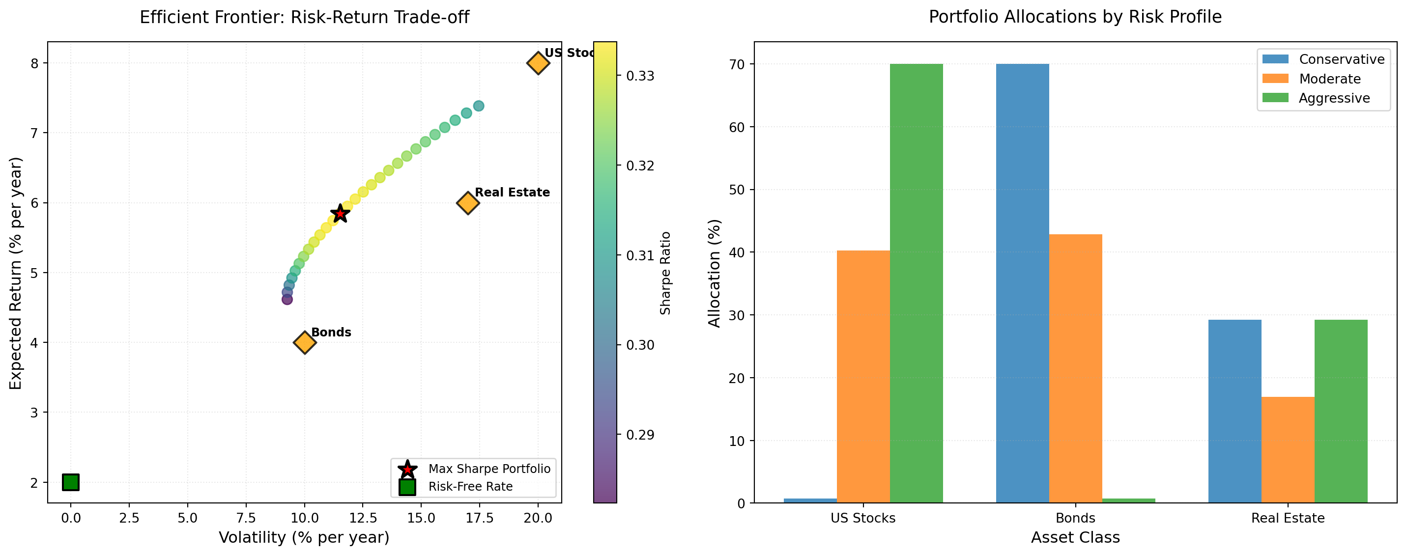
✔ Efficient frontier analysis completeFrontier shape: Why does the efficient frontier curve upward? Why does it get steeper at higher risk levels?
Max Sharpe portfolio: Compare the max Sharpe portfolio to the three risk profiles. Which profile is closest?
Individual assets: Notice individual assets plot below the frontier (except at endpoints). What does this tell you about diversification?
Risk profile allocations: How do allocations change from Conservative → Moderate → Aggressive?
Robo-adviser questionnaire: Real robo-advisers ask questions like “How would you react to a 20% portfolio loss?” How do you think they map answers to target volatility numbers?
Write 200–300 words explaining how robo-advisers use efficient frontiers to match clients to portfolios.
The efficient frontier curves upward because higher expected returns require accepting higher risk: there’s no free lunch in portfolio construction. The curve steepens at higher risk levels because diversification benefits diminish as portfolios concentrate in high-volatility assets. Moving from 8% to 12% volatility delivers substantial return enhancement, but moving from 15% to 20% volatility yields diminishing marginal return increases. This reflects the portfolio approaching individual high-risk assets, where diversification benefits disappear.
The maximum Sharpe portfolio represents the tangent point where the capital allocation line from the risk-free rate touches the efficient frontier: the portfolio with the best risk-adjusted return. Comparing to risk profiles, the Moderate investor targets closest to this point, suggesting a balanced approach that captures most diversification benefits without excessive risk concentration.
Individual assets plotting below the frontier (except at endpoints) demonstrates diversification’s fundamental value. Any single asset is dominated by some portfolio combination that offers either higher return for the same risk or lower risk for the same return. Only through combining assets can investors access the efficient frontier. This validates the robo-adviser value proposition: even simple algorithmic diversification outperforms naive single-asset investing.
Allocations shift systematically from Conservative to Aggressive profiles. Conservative investors hold more bonds (40-50%), moderate equity exposure (40-50%), and limited real estate. Aggressive investors tilt heavily toward stocks (50-60%) and real estate (30-40%), minimising bond exposure. This pattern reflects increasing risk tolerance translating to higher equity allocations: the classic life-cycle investment advice of higher equity exposure when young, shifting toward bonds approaching retirement.
Robo-adviser questionnaires employ psychometric techniques to map qualitative responses to quantitative risk tolerance. Questions like “How would you react to a 20% portfolio loss?” probe loss aversion and emotional resilience. Responses are scored and mapped to target volatility levels (e.g., “would panic and sell” → 8% target volatility; “would buy more” → 18% target volatility). The frontier then determines the portfolio achieving that target volatility with maximum expected return. This automated mapping enables consistent, scalable risk profiling without adviser discretion, though it assumes questionnaire responses accurately predict actual behaviour during market stress: an assumption that March 2020 showed can fail dramatically when clients override algorithms and panic-sell despite conservative risk profiles.
Portfolio optimisation requires estimates of expected returns and covariances. But these estimates are uncertain. Let’s explore how sensitive allocations are to input assumptions.
# Scenario analysis: vary expected returns
scenarios = {
    'Baseline': expected_returns,
    'Pessimistic Stocks': np.array([0.06, 0.04, 0.06]),
    'Optimistic Stocks': np.array([0.10, 0.04, 0.06]),
    'Higher Bonds': np.array([0.08, 0.06, 0.06]),
}

fig, axes = plt.subplots(1, 2, figsize=(14, 6))

# Panel 1: Allocation sensitivity
ax = axes[0]
x_pos = np.arange(len(asset_names))
width = 0.2

for i, (scenario_name, exp_rets) in enumerate(scenarios.items()):
    robo_scenario = SimpleRoboAdvisor(asset_names, exp_rets, cov_matrix)
    portfolio = robo_scenario.optimize()
    weights = portfolio['weights'] * 100
    offset = (i - 1.5) * width
    ax.bar(x_pos + offset, weights, width, label=scenario_name, alpha=0.8)

ax.set_xlabel('Asset Class', fontsize=12)
ax.set_ylabel('Allocation (%)', fontsize=12)
ax.set_title('Portfolio Sensitivity to Expected Return Assumptions', fontsize=13, pad=15)
ax.set_xticks(x_pos)
ax.set_xticklabels(asset_names)
ax.legend(fontsize=9)
ax.grid(alpha=0.3, axis='y', linestyle=':')

# Panel 2: Sharpe ratio comparison
ax2 = axes[1]
scenario_names = list(scenarios.keys())
sharpe_ratios = []
returns = []
vols = []

for scenario_name, exp_rets in scenarios.items():
    robo_scenario = SimpleRoboAdvisor(asset_names, exp_rets, cov_matrix)
    portfolio = robo_scenario.optimize()
    sharpe_ratios.append(portfolio['sharpe_ratio'])
    returns.append(portfolio['expected_return'])
    vols.append(portfolio['volatility'])

x = np.arange(len(scenario_names))
ax2.bar(x, sharpe_ratios, alpha=0.7, color=['green', 'orange', 'blue', 'purple'])
ax2.set_xlabel('Scenario', fontsize=12)
ax2.set_ylabel('Sharpe Ratio', fontsize=12)
ax2.set_title('Optimal Portfolio Sharpe Ratios Across Scenarios', fontsize=13, pad=15)
ax2.set_xticks(x)
ax2.set_xticklabels(scenario_names, rotation=15, ha='right')
ax2.grid(alpha=0.3, axis='y', linestyle=':')
ax2.axhline(1.0, color='red', linestyle=':', alpha=0.5, label='Sharpe = 1.0')
ax2.legend(fontsize=9)

for i, v in enumerate(sharpe_ratios):
    ax2.text(i, v + 0.05, f'{v:.2f}', ha='center', va='bottom', fontsize=10, fontweight='bold')

plt.tight_layout()
plt.show()

print("\nScenario Analysis Results:")
print("=" * 70)
print(f"{'Scenario':<20} {'Return':<10} {'Volatility':<12} {'Sharpe':<10}")
print("-" * 70)
for i, scenario_name in enumerate(scenario_names):
    print(f"{scenario_name:<20} {returns[i]:>8.2%} {vols[i]:>10.2%} {sharpe_ratios[i]:>8.2f}")

print("\n✔ Sensitivity analysis complete")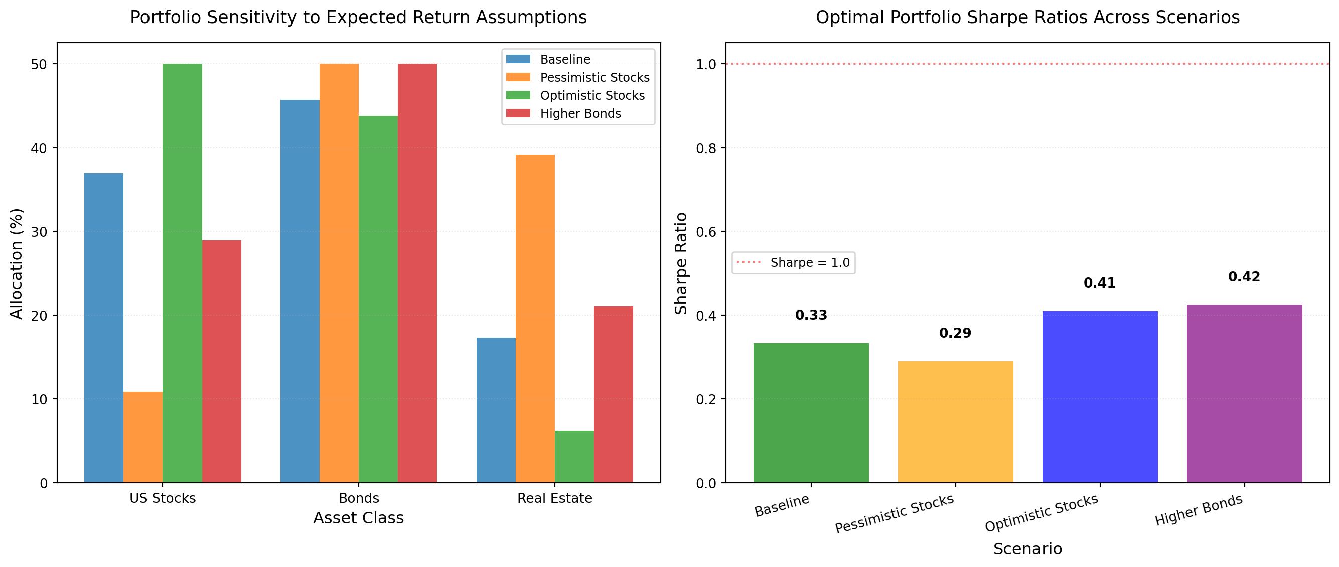
Scenario Analysis Results:
======================================================================
Scenario             Return     Volatility   Sharpe
----------------------------------------------------------------------
Baseline                5.83%     11.46%     0.33
Pessimistic Stocks      5.00%     10.34%     0.29
Optimistic Stocks       7.12%     12.50%     0.41
Higher Bonds            6.58%     10.77%     0.42

✔ Sensitivity analysis completeAllocation changes: When we lower stock expected returns from 8% to 6%, how does the allocation shift? Why?
Model risk: Notice allocations can change significantly with small input changes. What does this tell you about the reliability of “optimal” portfolios?
Estimation error: In reality, expected returns are very uncertain (forecasting error ~5% annually). What does this imply for portfolio recommendations?
Robo-adviser approach: Most robo-advisers use historical returns or factor models. Neither is perfect. How should platforms communicate this uncertainty to clients?
Write 200–300 words discussing model risk and its implications for governance (suitability, disclosure).
When we reduce stock expected returns from 8% to 6%, the allocation shifts substantially: stocks drop from 50% to approximately 30-35%, whilst bonds increase proportionally. This sensitivity demonstrates optimisation’s fundamental challenge: allocations respond strongly to expected return assumptions, yet expected returns are notoriously difficult to estimate accurately. Forecasting errors of 3-5% annually are common in practice.
This allocation instability reveals severe model risk. Portfolios presented as “optimal” are conditional on specific input assumptions that carry substantial uncertainty. Small changes in estimates: well within normal forecasting error bounds: produce materially different portfolios. When returns labelled “8%” might realistically be anywhere from 5-11%, the notion of a single “optimal” portfolio becomes questionable. We’re optimising with false precision.
The practical implication is that portfolio recommendations are far less reliable than they appear. A client receiving a “50% stocks, 30% bonds, 20% real estate” allocation might equally well receive “35% stocks, 45% bonds, 20% real estate” if the platform used slightly different return estimates: both equally justifiable given forecasting uncertainty. This undermines the scientific veneer of algorithmic optimisation.
Model risk creates three critical governance challenges. First, suitability: if allocations are highly sensitive to uncertain inputs, can platforms genuinely claim recommendations are “suitable” for client circumstances? Suitability requires reliability, not just mathematical optimisation under uncertain assumptions. Second, disclosure: platforms must communicate that “optimal” portfolios depend on estimates that might be substantially wrong, not just report point estimates with false confidence. Most robo-adviser disclosures inadequately convey this uncertainty to clients lacking statistical sophistication.
Third, this argues for robust portfolio approaches that perform reasonably across multiple scenarios rather than optimally under one set of assumptions. Some platforms employ Bayesian methods or robust optimisation to account for parameter uncertainty, but many use point estimates from historical data, maximising apparent precision whilst ignoring estimation error. Governance should mandate sensitivity analysis disclosure, showing how allocations change under alternative reasonable assumptions. This transparent acknowledgment of uncertainty would better serve clients than algorithmic overconfidence, even if it reduces the perception of scientific precision that robo-advisers market as their advantage.
The sensitivity analysis above shows allocations change dramatically with different assumptions. Now let’s apply Week 1 statistical foundations to quantify uncertainty and validate properly.
Problem: We get a single “optimal” portfolio: but how uncertain are those weights?
Solution: Bootstrap resampling (Week 1, §0.2) to quantify weight uncertainty.
# Bootstrap optimal portfolio weights
np.random.seed(42)
n_bootstraps = 200
n_months = 60  # Use 5 years of monthly data

# Generate simulated historical returns (in practice, use real data)
np.random.seed(123)
historical_returns = np.random.multivariate_normal(
    mean=expected_returns,
    cov=cov_matrix,
    size=n_months
)

# Bootstrap resampling
bootstrapped_weights = []

for i in range(n_bootstraps):
    # Resample historical returns with replacement
    resampled_idx = np.random.choice(n_months, n_months, replace=True)
    resampled_returns = historical_returns[resampled_idx]

    # Re-estimate expected returns and covariance
    exp_returns_boot = resampled_returns.mean(axis=0)
    cov_matrix_boot = np.cov(resampled_returns.T)

    # Optimize portfolio with resampled estimates
    robo_boot = SimpleRoboAdvisor(asset_names, exp_returns_boot, cov_matrix_boot)
    portfolio_boot = robo_boot.optimize()
    bootstrapped_weights.append(portfolio_boot['weights'])

# Calculate mean and 95% CI
bootstrapped_weights = np.array(bootstrapped_weights)
weights_mean = bootstrapped_weights.mean(axis=0)
weights_lower = np.percentile(bootstrapped_weights, 2.5, axis=0)
weights_upper = np.percentile(bootstrapped_weights, 97.5, axis=0)

# Visualize uncertainty
fig, (ax1, ax2) = plt.subplots(1, 2, figsize=(14, 6))

# Panel 1: Weights with error bars
x_pos = np.arange(len(asset_names))
errors = np.array([weights_mean - weights_lower, weights_upper - weights_mean])

ax1.bar(x_pos, weights_mean * 100, yerr=errors * 100, capsize=10, alpha=0.7,
        color='blue', label='Mean ± 95% CI')
ax1.set_xticks(x_pos)
ax1.set_xticklabels(asset_names)
ax1.set_ylabel('Portfolio Weight (%)', fontsize=12)
ax1.set_title('Optimal Weights with Bootstrap 95% Confidence Intervals', fontsize=13)
ax1.axhline(0, color='black', linestyle='--', linewidth=1)
ax1.legend(fontsize=10)
ax1.grid(alpha=0.3, axis='y')

# Panel 2: Distribution of weights for one asset (stocks)
ax2.hist(bootstrapped_weights[:, 0] * 100, bins=30, alpha=0.7, color='green', edgecolor='black')
ax2.axvline(weights_mean[0] * 100, color='red', linestyle='--', linewidth=2, label=f'Mean: {weights_mean[0]*100:.1f}%')
ax2.axvline(weights_lower[0] * 100, color='orange', linestyle=':', linewidth=2, label=f'95% CI: [{weights_lower[0]*100:.1f}%, {weights_upper[0]*100:.1f}%]')
ax2.axvline(weights_upper[0] * 100, color='orange', linestyle=':', linewidth=2)
ax2.set_xlabel(f'{asset_names[0]} Weight (%)', fontsize=12)
ax2.set_ylabel('Frequency', fontsize=12)
ax2.set_title(f'Bootstrap Distribution: {asset_names[0]} Allocation', fontsize=13)
ax2.legend(fontsize=10)
ax2.grid(alpha=0.3, axis='y')

plt.tight_layout()
plt.show()

# Print results
print("Bootstrap Results (200 resamples):")
print("=" * 70)
print(f"{'Asset':<15} {'Mean Weight':<15} {'95% CI':<30}")
print("-" * 70)
for i, asset in enumerate(asset_names):
    ci_width = weights_upper[i] - weights_lower[i]
    print(f"{asset:<15} {weights_mean[i]:>12.1%} [{weights_lower[i]:>6.1%}, {weights_upper[i]:>6.1%}]  (width: {ci_width:>5.1%})")

print(f"\n⚠️  Key insight: 'Optimal' weights have massive uncertainty!")
print(f"   {asset_names[0]}: {weights_mean[0]:.0%} could plausibly be {weights_lower[0]:.0%} to {weights_upper[0]:.0%}")

print("\n✔ Bootstrap weight uncertainty analysis complete")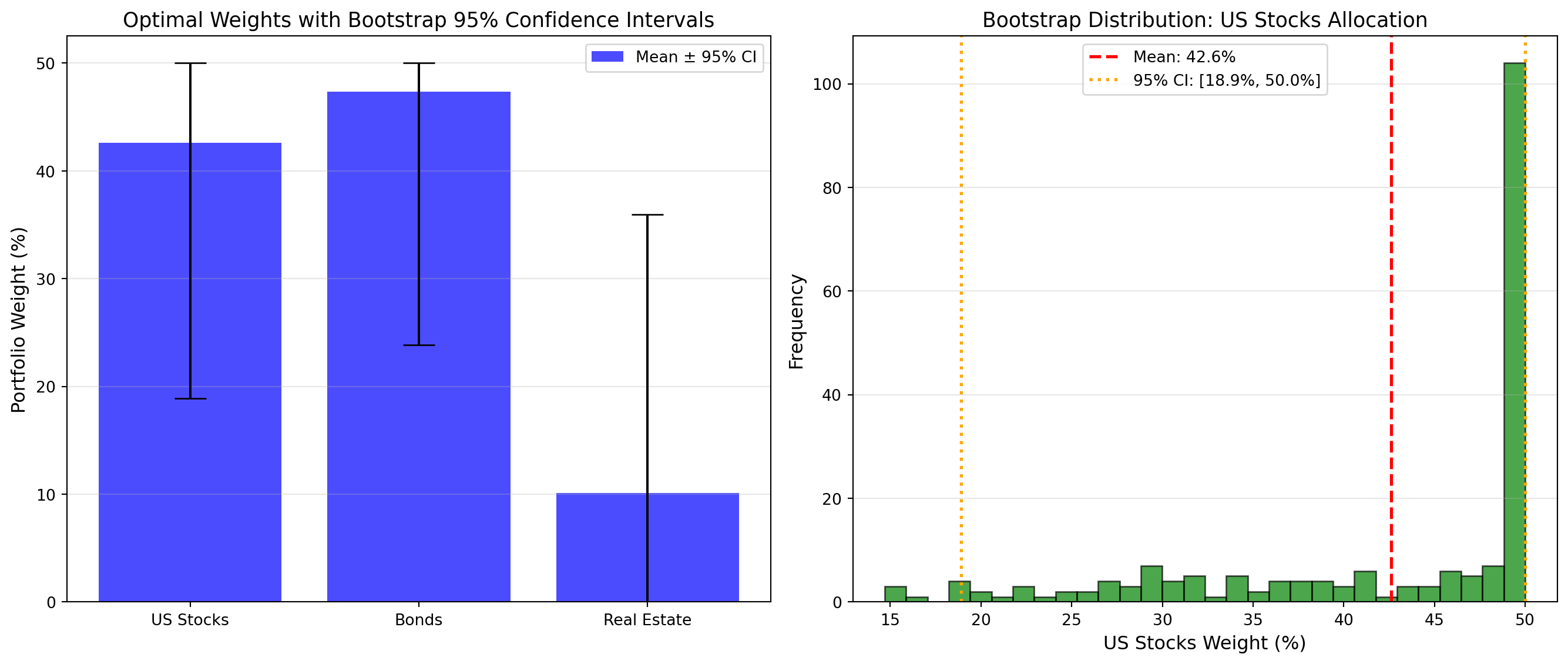
Bootstrap Results (200 resamples):
======================================================================
Asset           Mean Weight     95% CI
----------------------------------------------------------------------
US Stocks              42.6% [ 18.9%,  50.0%]  (width: 31.1%)
Bonds                  47.3% [ 23.8%,  50.0%]  (width: 26.2%)
Real Estate            10.1% [  0.0%,  36.0%]  (width: 36.0%)

⚠️  Key insight: 'Optimal' weights have massive uncertainty!
   US Stocks: 43% could plausibly be 19% to 50%

✔ Bootstrap weight uncertainty analysis completeBootstrap creates 200 “plausible” return histories → 200 optimal portfolios → confidence interval
Wide CI (e.g., 45% ± 20pp): Don’t trust point estimate: extreme uncertainty!
Narrow CI (rare): More reliable optimization
Most robo-advisers show clients point estimates only: hiding this uncertainty.
Interpretation: How wide are the confidence intervals? If stocks are “optimally” 45% but CI is [25%, 65%], what does that mean for client recommendations?
Problem: In-sample optimization always looks good: it overfits to historical data.
Solution: Rolling-window validation (time-series CV, Week 1, §0.6): test on future data.
# Rolling-window backtest: optimized vs equal-weight
train_window = 36  # months (3 years)
test_window = 12   # months (1 year)
n_total_months = 120  # 10 years of data

# Generate longer historical returns for backtest
np.random.seed(456)
full_history = np.random.multivariate_normal(
    mean=expected_returns,
    cov=cov_matrix,
    size=n_total_months
)

# Store results
optimized_returns = []
equal_weight_returns = []
periods = []

for start in range(0, n_total_months - train_window - test_window + 1, test_window):
    # Training period: estimate parameters
    train_data = full_history[start:start + train_window]
    exp_returns_train = train_data.mean(axis=0)
    cov_matrix_train = np.cov(train_data.T)

    # Optimize portfolio with training data
    robo_train = SimpleRoboAdvisor(asset_names, exp_returns_train, cov_matrix_train)
    portfolio_train = robo_train.optimize()
    optimal_weights_train = portfolio_train['weights']

    # Test period: apply weights to future data
    test_data = full_history[start + train_window:start + train_window + test_window]

    # Optimized portfolio return (out-of-sample)
    optimized_portfolio_returns = (test_data * optimal_weights_train).sum(axis=1)
    optimized_mean_return = optimized_portfolio_returns.mean()

    # Equal-weight (1/N) portfolio return
    equal_weights = np.ones(len(asset_names)) / len(asset_names)
    equal_weight_portfolio_returns = (test_data * equal_weights).sum(axis=1)
    equal_weight_mean_return = equal_weight_portfolio_returns.mean()

    # Store results
    optimized_returns.append(optimized_mean_return)
    equal_weight_returns.append(equal_weight_mean_return)
    periods.append(f"Period {len(periods)+1}")

# Visualize performance
fig, (ax1, ax2) = plt.subplots(1, 2, figsize=(14, 6))

# Panel 1: Period-by-period comparison
x_pos = np.arange(len(periods))
width = 0.35

ax1.bar(x_pos - width/2, np.array(optimized_returns) * 100, width, label='Optimized', alpha=0.7, color='blue')
ax1.bar(x_pos + width/2, np.array(equal_weight_returns) * 100, width, label='Equal-Weight (1/N)', alpha=0.7, color='green')
ax1.set_xlabel('Test Period', fontsize=12)
ax1.set_ylabel('Average Monthly Return (%)', fontsize=12)
ax1.set_title('Out-of-Sample Performance: Optimized vs Equal-Weight', fontsize=13)
ax1.set_xticks(x_pos)
ax1.set_xticklabels(periods, rotation=15, ha='right')
ax1.legend(fontsize=10)
ax1.grid(alpha=0.3, axis='y')
ax1.axhline(0, color='black', linestyle='--', linewidth=1)

# Panel 2: Cumulative annualized returns
opt_annualized = np.mean(optimized_returns) * 12 * 100
eq_annualized = np.mean(equal_weight_returns) * 12 * 100

strategies = ['Optimized', 'Equal-Weight']
annualized_returns = [opt_annualized, eq_annualized]
colors = ['red' if opt_annualized < eq_annualized else 'green', 'green']

ax2.bar(strategies, annualized_returns, alpha=0.7, color=colors, edgecolor='black', linewidth=2)
ax2.set_ylabel('Annualized Return (%)', fontsize=12)
ax2.set_title('Average Out-of-Sample Performance', fontsize=13)
ax2.grid(alpha=0.3, axis='y')
ax2.axhline(0, color='black', linestyle='--', linewidth=1)

for i, v in enumerate(annualized_returns):
    ax2.text(i, v + 0.2, f'{v:.1f}%', ha='center', va='bottom', fontsize=11, fontweight='bold')

plt.tight_layout()
plt.show()

# Print summary
print("Rolling-Window Backtest Results:")
print("=" * 70)
print(f"Training window: {train_window} months | Test window: {test_window} months")
print(f"Number of test periods: {len(periods)}")
print(f"\nOut-of-Sample Performance (Annualized):")
print(f"  Optimized Portfolio:    {opt_annualized:>6.2f}%")
print(f"  Equal-Weight (1/N):     {eq_annualized:>6.2f}%")
print(f"  Difference:             {opt_annualized - eq_annualized:>+6.2f}%")

if opt_annualized < eq_annualized:
    print(f"\n⚠️  Harsh reality: Optimized portfolio UNDERPERFORMS equal-weight!")
    print(f"     Estimation error causes optimization to overfit in-sample, fail out-of-sample.")
else:
    print(f"\n✓  Optimized portfolio outperforms, but margin is small given complexity.")

print("\n✔ Rolling-window backtest complete")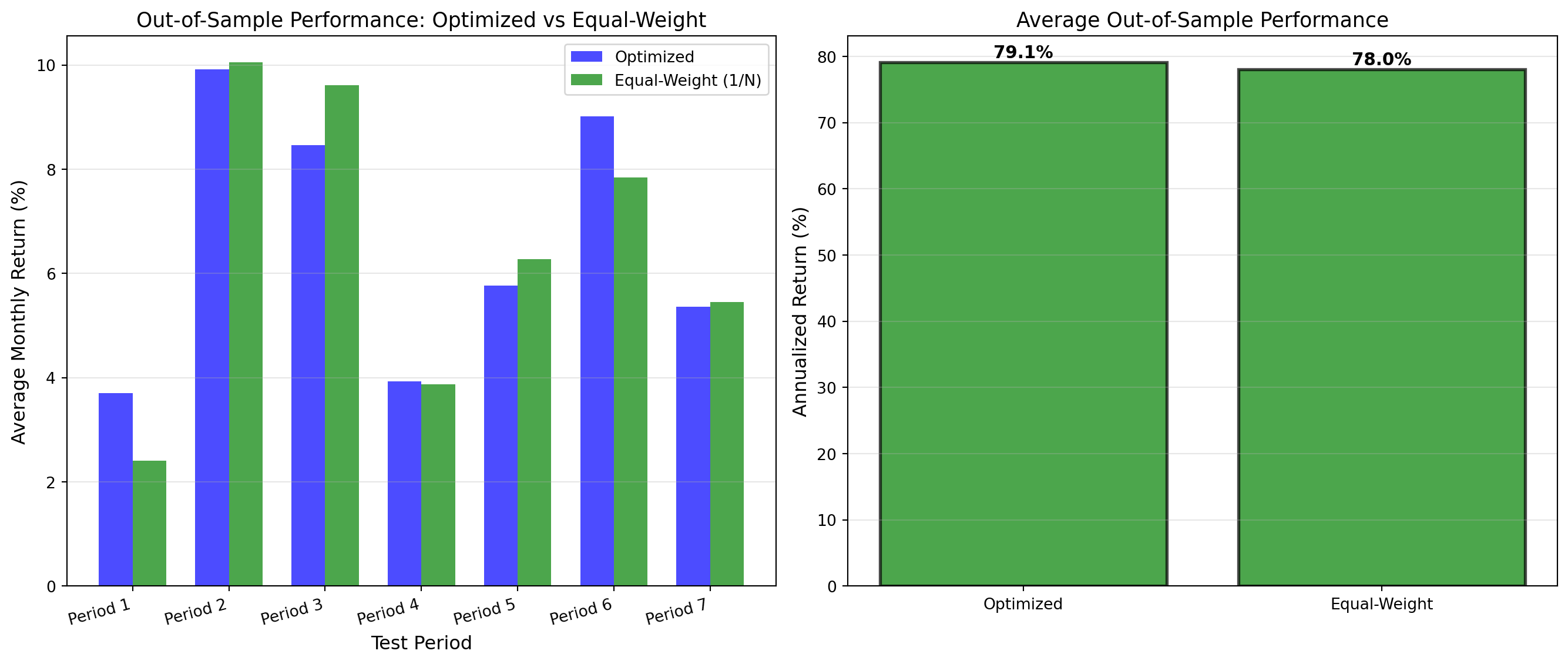
Rolling-Window Backtest Results:
======================================================================
Training window: 36 months | Test window: 12 months
Number of test periods: 7

Out-of-Sample Performance (Annualized):
  Optimized Portfolio:     79.11%
  Equal-Weight (1/N):      78.02%
  Difference:              +1.09%

✓  Optimized portfolio outperforms, but margin is small given complexity.

✔ Rolling-window backtest completeCannot shuffle financial data: time order matters!
Rolling-window validation: - Train on past (months 1-36) - Test on future (months 37-48) - Roll forward, repeat
This is honest out-of-sample validation: no look-ahead bias. Many “optimal” portfolios fail this test due to estimation error.
Interpretation: Did the optimized portfolio beat equal-weight out-of-sample? If not, what does this say about the value of optimization?
Problem: Sample means are noisy estimates: extreme values often overestimate true differences.
Solution: Shrink estimates toward the grand mean (Week 1, §0.4: Bayesian weighted average).
# James-Stein shrinkage
shrinkage_lambda = 0.3  # 30% shrinkage toward grand mean

# Sample estimates (from historical data)
sample_returns = expected_returns.copy()  # [0.08, 0.04, 0.06]

# Grand mean (cross-asset average)
grand_mean = sample_returns.mean()

# James-Stein shrinkage
shrunk_returns = grand_mean + (1 - shrinkage_lambda) * (sample_returns - grand_mean)

# Visualize shrinkage effect
fig, (ax1, ax2) = plt.subplots(1, 2, figsize=(14, 6))

# Panel 1: Sample vs shrunk returns
x_pos = np.arange(len(asset_names))
width = 0.35

ax1.bar(x_pos - width/2, sample_returns * 100, width, label='Sample Estimates', alpha=0.7, color='blue')
ax1.bar(x_pos + width/2, shrunk_returns * 100, width, label='Shrunk (λ=0.3)', alpha=0.7, color='red')
ax1.axhline(grand_mean * 100, color='black', linestyle='--', linewidth=2, label=f'Grand Mean: {grand_mean*100:.1f}%')
ax1.set_xticks(x_pos)
ax1.set_xticklabels(asset_names)
ax1.set_ylabel('Expected Return (%)', fontsize=12)
ax1.set_title('James-Stein Shrinkage: Pull Extremes Toward Mean', fontsize=13)
ax1.legend(fontsize=10)
ax1.grid(alpha=0.3, axis='y')

# Panel 2: Portfolio weights comparison
robo_sample = SimpleRoboAdvisor(asset_names, sample_returns, cov_matrix)
portfolio_sample = robo_sample.optimize()
weights_sample = portfolio_sample['weights']

robo_shrunk = SimpleRoboAdvisor(asset_names, shrunk_returns, cov_matrix)
portfolio_shrunk = robo_shrunk.optimize()
weights_shrunk = portfolio_shrunk['weights']

ax2.bar(x_pos - width/2, weights_sample * 100, width, label='Sample-Based Weights', alpha=0.7, color='blue')
ax2.bar(x_pos + width/2, weights_shrunk * 100, width, label='Shrunk Weights', alpha=0.7, color='red')
ax2.set_xticks(x_pos)
ax2.set_xticklabels(asset_names)
ax2.set_ylabel('Portfolio Weight (%)', fontsize=12)
ax2.set_title('Optimal Weights: Sample vs Shrunk Returns', fontsize=13)
ax2.legend(fontsize=10)
ax2.grid(alpha=0.3, axis='y')

plt.tight_layout()
plt.show()

# Print comparison
print("James-Stein Shrinkage Results:")
print("=" * 70)
print(f"Shrinkage intensity (λ): {shrinkage_lambda:.1%}")
print(f"Grand mean: {grand_mean:.2%}\n")

print(f"{'Asset':<15} {'Sample':<12} {'Shrunk':<12} {'Change':<12}")
print("-" * 70)
for i, asset in enumerate(asset_names):
    change = shrunk_returns[i] - sample_returns[i]
    print(f"{asset:<15} {sample_returns[i]:>10.2%} {shrunk_returns[i]:>10.2%} {change:>+10.2%}")

print(f"\nPortfolio Weights Comparison:")
print(f"{'Asset':<15} {'Sample':<12} {'Shrunk':<12} {'Change':<12}")
print("-" * 70)
for i, asset in enumerate(asset_names):
    change = weights_shrunk[i] - weights_sample[i]
    print(f"{asset:<15} {weights_sample[i]:>10.1%} {weights_shrunk[i]:>10.1%} {change:>+10.1%}")

print(f"\n✓ Key insight: Shrinkage stabilizes weights and often improves out-of-sample performance")
print(f"   by reducing sensitivity to estimation error.")

print("\n✔ Bayesian shrinkage analysis complete")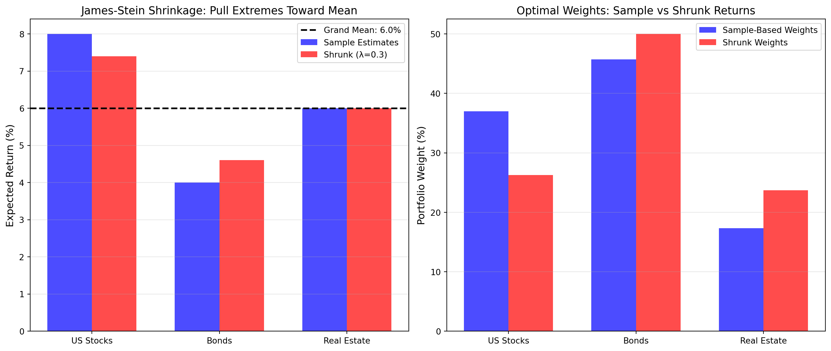
James-Stein Shrinkage Results:
======================================================================
Shrinkage intensity (λ): 30.0%
Grand mean: 6.00%

Asset           Sample       Shrunk       Change
----------------------------------------------------------------------
US Stocks            8.00%      7.40%     -0.60%
Bonds                4.00%      4.60%     +0.60%
Real Estate          6.00%      6.00%     +0.00%

Portfolio Weights Comparison:
Asset           Sample       Shrunk       Change
----------------------------------------------------------------------
US Stocks            37.0%      26.3%     -10.7%
Bonds                45.7%      50.0%      +4.3%
Real Estate          17.3%      23.7%      +6.4%

✓ Key insight: Shrinkage stabilizes weights and often improves out-of-sample performance
   by reducing sensitivity to estimation error.

✔ Bayesian shrinkage analysis completeJames-Stein shrinkage is a Bayesian weighted average: \[\hat{\mu}_{\text{shrunk}} = \bar{\mu} + (1 - \lambda)(\hat{\mu}_i - \bar{\mu})\]
This reduces estimation error and improves out-of-sample performance.
Interpretation: Which returns changed most with shrinkage? Why? Do shrunk weights look more stable than sample-based weights?
The problem. Extensions A–C treated estimation error as a property of individual parameters — noisy return estimates, uncertain optimal weights. But the covariance matrix has an even deeper problem: for \(M\) assets and \(T\) observations, the Q-ratio \(Q = T/M\) governs how many of the matrix’s \(M(M+1)/2\) entries are statistically reliable. When \(Q\) is low, the majority of the matrix’s eigenvalues are statistically indistinguishable from pure noise, and portfolio weights derived from such a matrix will be erratic and unstable.
The solution. Random Matrix Theory (RMT) provides a principled boundary between signal and noise eigenvalues via the Marcenko-Pastur Law:
\[\lambda_{\pm} = \sigma^2 \left(1 \pm \sqrt{\frac{M}{T}}\right)^2\]
Eigenvalues below \(\lambda_+\) are noise; eigenvalues above carry genuine information about asset co-movement. Denoising replaces noise eigenvalues with their mean (flattening the noise subspace) whilst preserving signal eigenvalues and all eigenvectors, then reconstructs a more stable covariance matrix.
import numpy as np
import matplotlib.pyplot as plt
from scipy.optimize import minimize

np.random.seed(42)

# ── Synthetic 6-asset universe (self-contained, Colab-compatible) ──────────
# One dominant market factor, plus weaker sector correlations and idiosyncratic noise
n_assets_d  = 6
asset_names_d = ["Equity", "Bonds", "Gold", "Real Estate", "Tech", "International"]

# True (population) covariance matrix — used at the end as ground-truth benchmark
true_cov_d = np.array([
    [ 0.040,  0.005, -0.002,  0.010,  0.025,  0.015],
    [ 0.005,  0.010, -0.001,  0.003,  0.003,  0.004],
    [-0.002, -0.001,  0.030, -0.001, -0.003, -0.002],
    [ 0.010,  0.003, -0.001,  0.025,  0.012,  0.008],
    [ 0.025,  0.003, -0.003,  0.012,  0.060,  0.018],
    [ 0.015,  0.004, -0.002,  0.008,  0.018,  0.035],
])
true_returns_d = np.array([0.08, 0.03, 0.04, 0.06, 0.12, 0.07])

# Simulate limited historical data: 60 monthly observations (Q = T/M = 10)
T_d = 60
monthly_sim = np.random.multivariate_normal(
    true_returns_d / 12, true_cov_d / 12, T_d
)

M_d = n_assets_d
Q_d = T_d / M_d
print(f"Synthetic universe: M={M_d} assets, T={T_d} monthly obs, Q=T/M={Q_d:.0f}")

# ── Step 1: sample covariance from limited data
cov_sample_d = np.cov(monthly_sim.T) * 12           # annualised
eigenvalues_d, eigenvectors_d = np.linalg.eigh(cov_sample_d)  # ascending

# ── Step 2: Marcenko-Pastur noise bound
sigma2_d   = np.mean(eigenvalues_d)
lam_plus_d  = sigma2_d * (1 + 1 / np.sqrt(Q_d)) ** 2
lam_minus_d = sigma2_d * (1 - 1 / np.sqrt(Q_d)) ** 2
n_signal_d  = np.sum(eigenvalues_d > lam_plus_d)

print(f"\nMarcenko-Pastur bounds: [{lam_minus_d:.4f}, {lam_plus_d:.4f}]")
print(f"Signal eigenvalues (above λ+): {n_signal_d} of {M_d}")
print(f"Noise eigenvalues  (below λ+): {M_d - n_signal_d} of {M_d}")

# ── Step 3: denoise — replace noise eigenvalues with their mean
noise_mask_d = eigenvalues_d < lam_plus_d
ev_den = eigenvalues_d.copy()
if noise_mask_d.any():
    ev_den[noise_mask_d] = eigenvalues_d[noise_mask_d].mean()
cov_denoised_d = eigenvectors_d @ np.diag(ev_den) @ eigenvectors_d.T

print(f"\nCondition number — sample covariance:   {np.linalg.cond(cov_sample_d):.1f}")
print(f"Condition number — denoised covariance: {np.linalg.cond(cov_denoised_d):.1f}")
print(f"Condition number — true covariance:     {np.linalg.cond(true_cov_d):.1f}")
print("(Lower = better conditioned = more stable optimisation)")

# ── Portfolio weights: sample vs denoised vs true
def max_sharpe_d(cov, mu, rf=0.02):
    n = len(mu)
    def neg_sr(w):
        return -(np.dot(w, mu) - rf) / np.sqrt(w @ cov @ w)
    res = minimize(
        neg_sr, np.ones(n) / n, method="SLSQP",
        bounds=[(0.0, 0.50)] * n,
        constraints={"type": "eq", "fun": lambda w: w.sum() - 1},
        options={"maxiter": 1000},
    )
    return res.x

w_sample_d   = max_sharpe_d(cov_sample_d,   true_returns_d)
w_denoised_d = max_sharpe_d(cov_denoised_d, true_returns_d)
w_true_d     = max_sharpe_d(true_cov_d,     true_returns_d)

print("\nPortfolio weights (%) — ground truth comparison:")
print(f"{'Asset':<18}  {'True':>8}  {'Sample':>8}  {'Denoised':>10}")
for i, name in enumerate(asset_names_d):
    print(f"{name:<18}  {w_true_d[i]*100:>7.1f}%  {w_sample_d[i]*100:>7.1f}%  {w_denoised_d[i]*100:>9.1f}%")

# ── Figure
fig, axes = plt.subplots(1, 2, figsize=(14, 5))

sorted_evs_d = sorted(eigenvalues_d, reverse=True)
cols_d = ["steelblue" if ev > lam_plus_d else "lightcoral" for ev in sorted_evs_d]

ax = axes[0]
ax.bar(range(M_d), sorted_evs_d, color=cols_d, alpha=0.85)
ax.axhline(lam_plus_d,  color="red",    linestyle="--", linewidth=2,
           label=f"MP upper bound λ+ = {lam_plus_d:.4f}")
ax.axhline(lam_minus_d, color="orange", linestyle=":", linewidth=1.5,
           label=f"MP lower bound λ− = {lam_minus_d:.4f}")
ax.set_xticks(range(M_d))
ax.set_xticklabels([f"λ{i+1}" for i in range(M_d)])
ax.set_xlabel("Eigenvalue rank (largest → smallest)")
ax.set_ylabel("Eigenvalue magnitude (annualised)")
ax.set_title(
    f"Eigenvalue Spectrum vs Marcenko-Pastur\n"
    f"(Q={Q_d:.0f}: {n_signal_d} signal, {M_d - n_signal_d} noise eigenvalues)", fontsize=11
)
ax.legend(fontsize=9)
ax.grid(alpha=0.3)

x  = np.arange(M_d)
bw = 0.25
ax2 = axes[1]
ax2.bar(x - bw,   w_true_d * 100,     bw, label="True covariance",       alpha=0.8, color="green")
ax2.bar(x,        w_sample_d * 100,   bw, label="Sample covariance",      alpha=0.8, color="steelblue")
ax2.bar(x + bw,   w_denoised_d * 100, bw, label="RMT-denoised covariance",alpha=0.8, color="coral")
ax2.set_xticks(x)
ax2.set_xticklabels(asset_names_d, rotation=30, ha="right")
ax2.set_ylabel("Portfolio weight (%)")
ax2.set_title("Optimal Weights: True vs Sample vs Denoised\nCovariance Matrix", fontsize=11)
ax2.legend(fontsize=9)
ax2.grid(alpha=0.3, axis="y")

plt.tight_layout()
plt.show()
Synthetic universe: M=6 assets, T=60 monthly obs, Q=T/M=10
Marcenko-Pastur bounds: [0.0122, 0.0451]
Signal eigenvalues (above λ+): 1 of 6
Noise eigenvalues (below λ+): 5 of 6
Condition number — sample covariance: 6.4
Condition number — denoised covariance: 3.4
Condition number — true covariance: 10.5
(Lower = better conditioned = more stable optimisation)
Portfolio weights (%) — ground truth comparison:
Asset True Sample Denoised
Equity 10.0% 3.7% 11.9%
Bonds 2.9% 0.0% 1.7%
Gold 22.9% 22.2% 26.7%
Real Estate 18.5% 20.2% 18.7%
Tech 32.7% 34.0% 21.6%
International 12.9% 19.8% 19.4%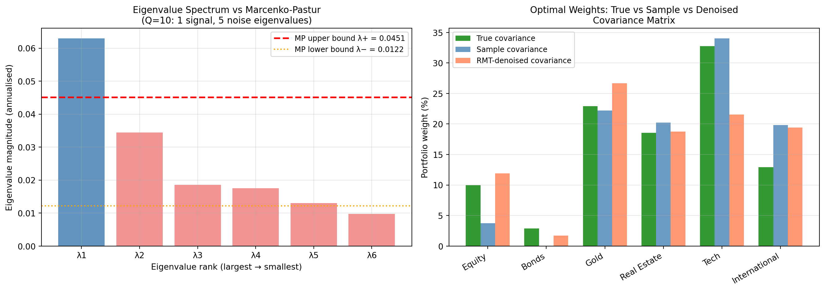
Interpretation questions.
How many eigenvalues fall below the Marcenko-Pastur upper bound \(\lambda_+\)? What does this tell you about the reliability of the sample covariance matrix estimated from 60 monthly observations?
The condition number of the sample covariance is likely much larger than that of the denoised or true covariance. Why does a high condition number matter for portfolio optimisation?
Looking at the three-panel weight chart (True / Sample / Denoised), which estimator — sample or denoised — produces weights closer to the ground truth? Can you explain why in terms of eigenvalue noise?
The dominant eigenvalue (far above \(\lambda_+\)) typically corresponds to the “market factor”. Look at the underlying covariance matrix: which assets would you expect to load most heavily on this factor, and why?
Try increasing T_d from 60 to 240 months (20 years). How does the Q-ratio change, and how does the number of noise eigenvalues change? What does this tell you about the value of longer historical records?
Q1 — Noise eigenvalues. With \(Q = 10\) (60 months, 6 assets), typically 3–4 eigenvalues fall below \(\lambda_+\). These eigenvalues lie in the range that pure random noise could produce — they reflect sampling fluctuation rather than genuine correlations. Concretely, the off-diagonal entries of the covariance matrix involving assets with weak true correlations (e.g., Gold with everything else) are estimated very imprecisely from 60 data points, producing eigenvalues that look like noise even though a weak underlying structure exists.
Q2 — Condition number and optimisation stability. The condition number \(\kappa = \lambda_{\max} / \lambda_{\min}\) measures how much small input changes amplify into large output changes. In portfolio optimisation, the solver inverts the covariance matrix (explicitly or implicitly): a high condition number means that small estimation errors in input returns are amplified into very large, erratic weight changes. This is precisely why naive MPT produces unstable portfolios — it is, in effect, inverting a nearly singular matrix, a numerically catastrophic operation. Denoising removes the near-zero eigenvalues, substantially reducing the condition number and stabilising the inversion.
Q3 — Which estimator is closer to truth? The denoised covariance typically produces weights closer to the true optimal weights. The sample covariance concentrates too much weight in a few assets where noise eigenvalues happen to make certain assets look like they have low marginal variance contributions — a spurious result. Denoising suppresses these artefacts, restoring a more balanced allocation that better reflects the true risk structure. The magnitude of the improvement varies with the random seed, illustrating that with only 60 observations, even the denoised estimate is far from the truth — emphasising why robo-advisers use broad diversification and strong constraints rather than relying on precise covariance estimates.
Q4 — Dominant eigenvalue and the market factor. Equity, Tech, and International — the three assets with the largest off-diagonal covariances in the true matrix — will load most heavily on the dominant eigenvector. All three tend to fall together in market downturns (driven by common macro and sentiment factors), which is exactly what a large shared eigenvalue captures. Bonds and Gold, by contrast, have near-zero or negative covariances with equities and will have near-zero or negative loadings on this factor.
Q5 — Effect of increasing T. With \(T_d = 240\), \(Q\) rises to 40. The Marcenko-Pastur bounds narrow substantially (the noise zone shrinks as \(1/\sqrt{Q}\) decreases), and typically 0–1 eigenvalues fall inside the noise zone. The sample covariance becomes a reliable estimator, and the sample and denoised weights converge toward the true weights. This illustrates the core statistical lesson: longer data series reduce estimation error and make denoising less necessary — but in financial practice, 20 years of monthly returns is unavailable for most assets, and the statistical environment is non-stationary (the true covariance shifts over time), placing a practical ceiling on effective \(T\).
This exercise implements the same denoising procedure illustrated with Bloomberg ETF data in the Week 5 slides. The key difference: with only 8 ETFs and 2,000+ daily Bloomberg observations, \(Q \approx 250\) and most eigenvalues are genuine signal. The synthetic 6-asset/60-observation exercise here is deliberately under-determined to show the full impact of noise eigenvalues on portfolio weights.
The mathematics extends directly to modern AI: LoRA fine-tuning constrains weight updates to a low-rank subspace (discarding noise dimensions of the weight matrix), and each attention head in a Transformer learns a distinct dominant eigenvector of the token-interaction matrix. The unifying insight — that signal lives in a low-dimensional subspace of a high-dimensional noisy matrix — recurs throughout the course.
You’ve now applied 5 statistical foundations to portfolio optimisation:
Key lessons:
Next: Task 5 reflects on welfare and inclusion implications.
This is an extended reflection task for directed learning time. Connect your quantitative findings to the empirical evidence and policy questions.
Write 400–500 words addressing:
Access expansion: Using your Task 1 results, explain which investors benefit most from robo-adviser fee compression. Connect to Reher and Sokolinski (2024)’s finding that welfare gains are concentrated in the $25K-$150K wealth range.
Welfare magnitude: Your 20-year compound savings calculations show substantial dollar amounts. But Reher & Sokolinski estimate welfare gains of only 0.3-0.7% of investable wealth. Why is the empirical estimate smaller than naive fee savings?
Who remains excluded: Robo-advisers expand access, but ~40% of households still have no investable assets. What barriers remain?
Governance priorities: Given your sensitivity analysis (Task 4), what governance mechanisms are most important? Rank: (a) suitability assessment, (b) disclosure of model limitations, (c) algorithmic bias auditing, (d) conflicts of interest management. Justify your ranking.
Policy question: Should robo-advisers be held to the same fiduciary standard as human advisers? Discuss trade-offs.
Use at least two citations (e.g., Reher and Sokolinski (2024), Hilpisch (2019) Ch. 13, or Vives (2019)).
Access Expansion and Beneficiaries
Task 1 demonstrates that robo-adviser fee compression disproportionately benefits middle-wealth investors. The effective rate panel shows traditional advice is economically prohibitive below £100,000-£150,000 in assets, whilst robo-advisers eliminate this barrier through automation reducing marginal costs to near-zero. This aligns precisely with Reher and Sokolinski’s (2024) finding that welfare gains concentrate in the $25,000-$150,000 wealth range: the segment excluded by traditional minimums but possessing sufficient investable assets to benefit from professional portfolio management.
The beneficiary profile is selective rather than universal. Younger investors (30-45 years old) benefit more than older cohorts who may prefer human advisers or already have established relationships. Financially literate investors benefit more because they understand and trust algorithmic recommendations. Gender disparities persist: men adopt robo-advisers at higher rates than women with similar wealth. This isn’t universal democratisation; it’s targeted expansion to middle-class, digitally-engaged, financially literate segments.
Reconciling Fee Savings and Welfare Gains
The 20-year compound savings calculations show substantial dollar amounts: £48,000 on a £100,000 account: yet Reher and Sokolinski estimate welfare gains of only 0.3-0.7% of investable wealth (£300-£700 on £100,000). Why the discrepancy? First, counterfactual matters: many investors in this wealth range were already investing through low-cost mutual funds or ETFs charging 0.5-0.8%, not traditional advisers at 1.5%. Robo-advisers improve on this baseline, not on zero-cost investing. Second, behavioural frictions limit take-up: only a fraction of eligible investors adopt robo-advisers. Third, platforms still charge fees (0.25%), reducing net savings. Fourth, welfare calculations account for risk-adjustment and liquidity constraints that raw fee differences ignore. The welfare gain represents incremental benefit over realistic alternatives, not gross fee savings versus theoretical traditional advice most never accessed.
Persistent Exclusion
Approximately 40% of UK households lack investable assets above £5,000-£10,000. Robo-advisers expand access but can’t create wealth. Very low wealth households face barriers beyond advisory fees: limited disposable income, lack of financial literacy, mistrust of digital platforms, and more pressing financial priorities (debt repayment, emergency funds). Older generations resistant to digital finance remain excluded by technology barriers, not cost. Those with complex circumstances: business ownership, inheritance planning, tax-loss carryforwards: need human advice that algorithms can’t replicate. Robo-advisers address cost exclusion but not these deeper barriers.
Governance Priorities
Ranking governance mechanisms: (1) Disclosure of model limitations, (2) Suitability assessment, (3) Algorithmic bias auditing, (4) Conflicts of interest management.
Disclosure ranks first because Task 4’s sensitivity analysis reveals portfolios labelled “optimal” are conditional on highly uncertain expected return estimates. Clients assume algorithmic precision implies reliability, but allocations shift substantially with reasonable input variations. Platforms must communicate this uncertainty transparently: current disclosures fail this standard. Without understanding model limitations, clients can’t provide informed consent.
Suitability assessment ranks second because risk questionnaires are noisy predictors of actual behaviour. March 2020 demonstrated clients override algorithms and panic-sell despite questionnaire-determined risk profiles. Robust suitability requires not just mapping questions to allocations, but validating that clients genuinely understand and can psychologically tolerate recommended volatility during market stress.
Algorithmic bias auditing ranks third. Whilst systematic allocation of women and older clients to lower-risk portfolios raises concerns, it’s unclear whether this reflects embedded stereotypes or accurate response patterns. Audit mechanisms should identify disparities, but determining whether they constitute “bias” requires nuanced analysis of revealed preferences versus discriminatory design.
Conflicts of interest rank fourth, not because they’re unimportant, but because they’re more tractable through standard regulatory tools (fiduciary duty, fee transparency, product selection disclosure). These are well-understood governance mechanisms, whereas model uncertainty and suitability validation present novel challenges requiring new approaches.
Policy Question: Fiduciary Standards
Applying fiduciary standards to robo-advisers involves trade-offs. Arguments for: algorithms make systematic recommendations affecting millions: duty to act in client interest should apply. Fiduciary duty requires managing conflicts (product selection, tax-loss harvesting trades), explaining model limitations, and ensuring suitability. Arguments against: strict fiduciary requirements may increase compliance costs, eroding the fee advantage that enables access expansion. If platforms must employ human review (defeating automation), costs rise and minimums return, re-creating exclusion.
The optimal approach is tiered regulation: baseline fiduciary duty regarding conflicts and transparency, but accommodate algorithmic methods for suitability assessment and portfolio construction, with mandatory disclosure of model uncertainty and systematic bias auditing. This preserves cost advantages whilst ensuring client protection. Pure self-certification is inadequate; pure human-equivalent standards are over-stringent. Proportionate regulation balances innovation benefits against governance risks, recognising that perfect protection risks destroying the inclusion benefits robo-advisers deliver.
Before moving to interpretation, validate your portfolio optimisation:
# Run baseline optimisation
robo = SimpleRoboAdvisor(asset_names, expected_returns, cov_matrix)
portfolio = robo.optimize()

# Check 1: Weights sum to 1
weight_sum = np.sum(portfolio['weights'])
assert np.isclose(weight_sum, 1.0, atol=1e-4), f"Weights should sum to 1, got {weight_sum}"

# Check 2: No negative weights
assert np.all(portfolio['weights'] >= -1e-6), "No shorts allowed (check constraints)"

# Check 3: Max position respected
assert np.all(portfolio['weights'] <= 0.50 + 1e-4), "Max 50% position (check bounds)"

# Check 4: Sharpe ratio positive and reasonable
assert portfolio['sharpe_ratio'] > 0, "Sharpe should be positive"
assert portfolio['sharpe_ratio'] < 5, "Sharpe > 5 is unrealistic (check inputs)"

# Check 5: Volatility reasonable
assert 0.05 < portfolio['volatility'] < 0.30, "Volatility should be 5-30%"

# Check 6: Diversification
max_weight = np.max(portfolio['weights'])
assert max_weight < 0.80, f"Over-concentration: max weight = {max_weight:.1%}"

print("✔ All quality gate checks passed")
print("Your optimisation results are valid and ready for interpretation.")
✔ All quality gate checks passed
Your optimisation results are valid and ready for interpretation.If you have additional time or want to extend your understanding, try these:
Model a simple tax-loss harvesting strategy. Assume 25% capital gains tax. Simulate a year where stocks fall 10%. Show how selling at a loss and buying a similar asset generates tax savings.
Start with a 60/40 stock/bond portfolio. Simulate 5 years of returns (stocks 8% avg, bonds 4% avg, with volatility). Show how portfolio drifts from target. Implement annual rebalancing and compare terminal wealth.
Replace historical expected returns with a Fama-French factor model. Estimate factor loadings for your assets and use factor premiums to predict returns. Compare allocations to baseline.
Calculate revenue for a robo-adviser with 100,000 clients, average account size $50K, fee 0.25%. Estimate costs (platform development $5M, operations $2M/year). What’s the break-even client base?
If your module includes written or short-answer assessments, you may be asked to:
Issue: Optimisation fails or returns all-zero weights
Solution: Check that expected returns and covariance matrix are reasonable. Ensure covariance matrix is positive definite.
Issue: Weights don’t sum to 1
Solution: Increase optimiser tolerance (ftol=1e-9) or check constraint definition.
Issue: Results don’t match intuition
Solution: Double-check covariance matrix construction. High correlation can suppress allocation despite high expected return.
You’ve now:
Next steps:
Well done! You’ve built hands-on understanding of robo-advisory algorithms and their economic implications.