---
title: "Data and Measurement in Finance"
subtitle: "Understanding Where Your Numbers Come From"
author: "Professor Barry Quinn"
date: today
format:
html:
code-fold: true
code-summary: "Show Python code"
code-tools:
source: true
toggle: true
caption: none
execute:
warning: false
message: false
echo: true
eval: true
fig-width: 10
fig-height: 6
fig-format: png
jupyter: fin510
bibliography:
- ../resources/reading.bib
- ../resources/reading_supp.bib
---
**Theme**: Data Foundations for Financial Analysis
::: {.callout-note}
#### View Slides
Open the lecture deck: [Week 2: Data and Measurement](../slides/week02_data.qmd)
:::
# Introduction: Why Data Understanding Matters
Before fitting any model : before running any regression, building any trading strategy, or training any algorithm : you need to understand where your data comes from. This is not merely a technical prerequisite; it is a basic scientific practice that separates rigorous analysis from uncritical “plug-and-play” statistics.
@gelman2020regression put it bluntly: "Before fitting a model... it is a good idea to understand where your numbers are coming from." This chapter develops that idea systematically, drawing on foundations from statistics, econometrics, and machine learning to build a framework for thinking critically about financial data.
The stakes are high. In finance, data problems don't just lead to poor academic papers : they lead to real losses, regulatory failures, and misallocated capital. A hedge fund that backtests on survivorship-biased data will overestimate returns. A risk model trained on crisis-free periods will underestimate tail risks. An algorithmic trading system that leaks future information into training will fail catastrophically in production.
::: {.callout-note}
## The Data Mindset
Understanding data is not a preliminary step to be rushed through before the "real" analysis. It *is* the analysis. The most sophisticated model built on flawed data will produce flawed results : often with false confidence.
:::
```{python}
#| label: setup-data-root
#| include: false
import sys
from pathlib import Path
sys.path.insert(0, str(Path("scripts").resolve()))
from bloomberg_loader import load_bloomberg
```
::: {.callout-tip}
## Simulations and Labs
Throughout this chapter, we use **simulated data** to illustrate concepts. These simulations are calibrated to match the **stylised facts** of real financial data : fat tails, volatility clustering, and realistic correlation structures. This approach lets us demonstrate principles cleanly without data access constraints.
In the **accompanying labs**, you'll work with **real data from Bloomberg Terminal** to see these concepts in action with all the messiness of actual markets. The labs complement this chapter by grounding theory in practice.
:::
## Learning Objectives
By the end of this chapter, you should be able to:
1. **Articulate** the data generating process (DGP) underlying a financial dataset
2. **Distinguish** between what you observe (measured variables) and what you want to understand (latent constructs)
3. **Identify** common selection biases in financial data and their consequences
4. **Apply** exploratory data analysis techniques appropriate for financial returns
5. **Implement** data validation procedures that catch quality issues before they affect analysis
# Part I: Where Data Come From
## The Data Generating Process Perspective
Every dataset is the output of some process : a **data generating process** (DGP) : that determines what gets recorded, when, and how. Understanding this process is essential because it reveals the assumptions embedded in your data before you add any modelling assumptions.
Consider stock price data. The prices you observe are not simply "the market" : they are the result of exchange mechanisms (how orders are matched and which prices are recorded), data vendor processing (how raw tick data is aggregated, cleaned, and distributed), selection rules (which securities are included in a database and for how long), and timing conventions (whether you see close, adjusted close, or bid-ask midpoint). Each of these choices affects your downstream analysis. Using unadjusted prices instead of split-adjusted prices will create spurious jumps. Using closing prices instead of volume-weighted average prices (VWAP) will introduce noise from end-of-day effects.
::: {.callout-tip}
## The Fundamental Question
Before any analysis, ask: "What mechanism produced these numbers, and how might that mechanism affect my conclusions?"
:::
### A Concrete Example: The Human Development Index
@gelman2020regression illustrate this principle with a non-financial example that has direct parallels to finance. The Human Development Index (HDI) was presented as a sophisticated measure of state-level development, but closer examination revealed:
> "The map in Figure 2.1 is pretty much a map of state income with a mysterious transformation and a catchy name. The relevance of this example is that we were better able to understand the data by plotting them in different ways."
The lesson? A variable with an impressive name may be largely driven by one simple component. In finance, this happens constantly: "smart beta" funds may be mostly driven by simple value or momentum tilts, "alternative data" signals may be proxying for publicly available information, and "risk-adjusted returns" depend entirely on how risk is measured. Always ask: what is this variable *actually* measuring, and is that what I think it's measuring?
## Selection Bias in Financial Data
Selection bias occurs when the data you have is systematically different from the population you want to study. In finance, several forms are endemic:
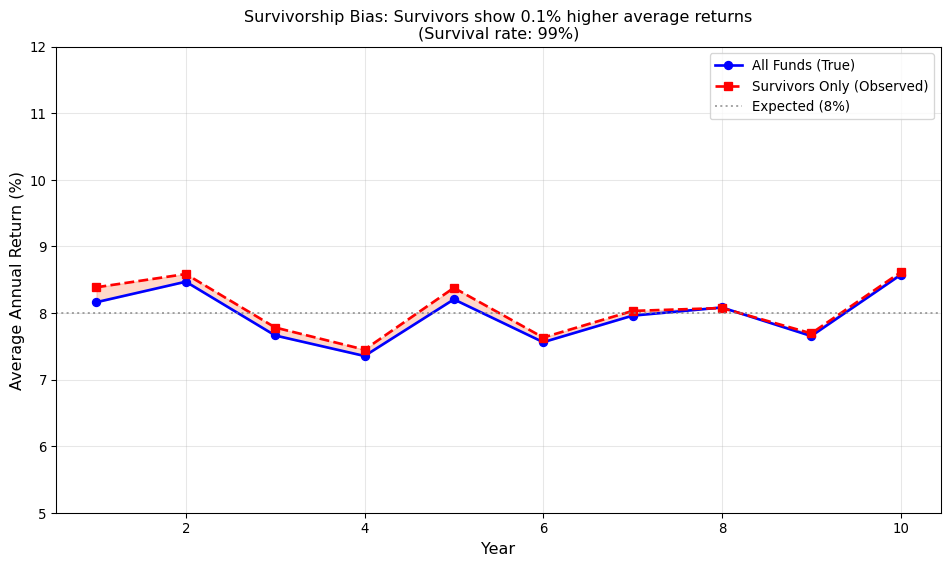
### Survivorship Bias
Databases of currently listed stocks exclude companies that failed, were acquired, or delisted. This creates an upward bias in measured returns because the worst performers have been removed.
| Study Type | Survivorship Impact | Typical direction |
|------------|---------------------|----------------|
| Mutual fund performance | Funds that close (often poor performers) disappear | Upward |
| Stock return analysis | Delisted firms (often bankruptcies) excluded | Upward |
| Hedge fund returns | Failed funds stop reporting | Upward (often large; hard to quantify) |
**Availability bias** arises because free and low-cost data sources have better coverage for large, liquid, well-known securities; analysis based only on easily available data may not generalise to the broader market. **Reporting bias** appears when companies and funds choose when and what to report : voluntary disclosures may be strategically timed, and self-reported hedge fund returns are particularly suspect because reporting is optional.
### Look-Ahead Bias
This is perhaps the most insidious form of selection in backtesting. It occurs when information that wasn't available at the time is used to make decisions. Common sources include point-in-time violations (using restated financial data rather than originally reported values), index membership (knowing which stocks will be added to an index before the announcement), and universe selection (selecting securities based on characteristics known only later).
::: {.callout-important}
## The Golden Rule of Backtesting
At any point in your backtest, you may only use information that was available at that point in time. This sounds obvious but is surprisingly easy to violate.
:::
### Quantifying Selection Bias
How large are these biases in practice? Research suggests they are economically meaningful:
```{python}
#| label: selection-bias-illustration
#| fig-cap: "Illustration of survivorship bias in fund returns"
#| eval: true
import numpy as np
import matplotlib.pyplot as plt

# Simulate fund returns with survivorship bias
np.random.seed(42)
n_funds = 1000
n_years = 10

# Generate true returns (some funds will fail)
true_returns = np.random.normal(0.08, 0.15, (n_funds, n_years))

# Funds with cumulative returns below -50% "fail" and stop reporting
cumulative = np.cumprod(1 + true_returns, axis=1)
failed = cumulative.min(axis=1) < 0.5
survival_rate = 1 - failed.mean()

# Calculate average returns: all funds vs survivors only
all_funds_mean = true_returns.mean(axis=0)
survivors_mean = true_returns[~failed].mean(axis=0)

# Plot
fig, ax = plt.subplots(figsize=(10, 6))
years = np.arange(1, n_years + 1)
ax.plot(years, all_funds_mean * 100, 'b-', lw=2, marker='o', label='All Funds (True)')
ax.plot(years, survivors_mean * 100, 'r--', lw=2, marker='s', label='Survivors Only (Observed)')
ax.axhline(y=8, color='gray', linestyle=':', alpha=0.7, label='Expected (8%)')
ax.fill_between(years, all_funds_mean * 100, survivors_mean * 100, alpha=0.3, color='coral')
ax.set_xlabel('Year', fontsize=12)
ax.set_ylabel('Average Annual Return (%)', fontsize=12)
ax.set_title(f'Survivorship Bias: Survivors show {(survivors_mean.mean() - all_funds_mean.mean())*100:.1f}% higher average returns\n(Survival rate: {survival_rate:.0%})', fontsize=12)
ax.legend(loc='upper right')
ax.grid(alpha=0.3)
ax.set_ylim(5, 12)
plt.tight_layout()
plt.show()

print(f"\nSimulation Summary:")
print(f"  Funds simulated: {n_funds}")
print(f"  Survival rate: {survival_rate:.1%}")
print(f"  True average return: {all_funds_mean.mean()*100:.2f}%")
print(f"  Observed (survivors): {survivors_mean.mean()*100:.2f}%")
print(f"  Survivorship bias: +{(survivors_mean.mean() - all_funds_mean.mean())*100:.2f}%")
```
::: {.callout-note}
## In-Class Lab: Real-World Survivorship Bias
In the **in-class Bloomberg lab**, we examine survivorship bias using **real UK banking data** from the 2008 financial crisis. You'll extract data from Bloomberg for Northern Rock, Bradford & Bingley, and HBOS : banks that failed or were rescued : and compare returns with and without these firms. The results are sobering: survivorship bias in UK banking returns during this period far exceeds what our simulation suggests.
**Before class**: Complete the [homework exercise](../labs/lab02_apis.qmd) to practice pipeline concepts with yfinance.
**In class**: [Lab 02: Survivorship Bias in UK Banking](../labs/lab02_survivorship_bias_bloomberg.qmd) (Bloomberg Terminal)
:::
# Part II: Validity and Reliability
## Measurement vs Latent Variables
A fundamental distinction in data science is between what we can **observe** (measured variables) and what we actually want to **understand** (latent variables or constructs). In finance, many of the concepts we care about cannot be directly observed:
| Latent Construct | Common Proxies | Measurement Issues |
|------------------|----------------|-------------------|
| **Market risk** | Beta, VaR, volatility | Different proxies capture different aspects |
| **Firm quality** | ROE, Tobin's Q, credit ratings | Accounting choices affect measurement |
| **Investor sentiment** | Surveys, put-call ratios, fund flows | Noisy, often contradictory |
| **Liquidity** | Bid-ask spread, volume, price impact | Multi-dimensional, context-dependent |
| **Information asymmetry** | PIN, analyst dispersion | Model-dependent |
The gap between construct and measurement matters because proxies are imperfect (market beta estimated from 60 months of data is a noisy estimate of true systematic risk), different proxies give different answers (book-to-market and earnings-to-price both proxy for "value" but behave differently), and measurement error biases regression coefficients (classic attenuation bias pushes coefficients toward zero).
@gelman2020regression emphasise this in their discussion of **validity** : does your measurement actually capture the construct you care about?
::: {.callout-note}
## Validity vs Reliability
**Validity** asks: "Am I measuring the right thing?"
**Reliability** asks: "Am I measuring it consistently?"
A measure can be reliable without being valid (consistently measuring the wrong thing), but it cannot be valid without being reliable (you can't accurately measure something if your measurements are all over the place).
:::
## Construct Validity in Finance
Construct validity asks whether our measurements actually capture the underlying concepts we intend to study. Consider the CAPM beta:
**The construct**: Systematic risk exposure : how much a stock moves with the market.
**The measurement**: Slope coefficient from regressing stock returns on market returns.
Validity concerns include which market index (S&P 500, CRSP, global equity), which time period (rolling 60 months, expanding window), which frequency (daily, weekly, monthly), and which return type (simple, log, excess). Different choices give different betas : sometimes very different. A stock might appear "defensive" (low beta) using monthly data but "aggressive" (high beta) using daily data due to different sensitivities to different types of market movements.
## Reliability: Would You Get the Same Answer Twice?
Reliability concerns whether measurements are consistent and reproducible. In finance, several factors affect reliability: sample period sensitivity (results that depend heavily on specific start/end dates), outlier sensitivity (conclusions that change dramatically with a few extreme observations), and specification sensitivity (results that flip sign with minor model changes). A reliable finding should be robust to reasonable variations in measurement and specification.
### The Attenuation Problem
When we use a noisy proxy for a true variable of interest, regression coefficients are biased toward zero. This is **attenuation bias** : the noisier the proxy, the more the coefficient is attenuated.
Mathematically, if we want to estimate $\beta$ in $y = \alpha + \beta x^* + \varepsilon$ but we only observe $x = x^* + u$ (where $u$ is measurement error), then OLS gives us:
$$\hat{\beta}_{OLS} = \beta \cdot \frac{\text{Var}(x^*)}{\text{Var}(x^*) + \text{Var}(u)}$$
The ratio is always less than 1, so $|\hat{\beta}_{OLS}| < |\beta|$. The more measurement error (larger $\text{Var}(u)$), the worse the attenuation.
**Finance implication**: Studies using noisy proxies for risk, sentiment, or information asymmetry will systematically underestimate the true relationships. This is one reason why "anomalies" often weaken when examined more carefully : better measurement reveals that the original effect was partially a measurement artefact.
# Part III: Exploratory Data Analysis
## The Philosophy of EDA
John Tukey's philosophy of **exploratory data analysis** (EDA) emphasises looking at data before modelling it. The goal is to understand distributional properties, identify patterns and relationships, detect anomalies and outliers, and generate hypotheses (rather than test them). @gelman2020regression express this as "all graphs are comparisons" : every visualisation should help you compare something meaningful.
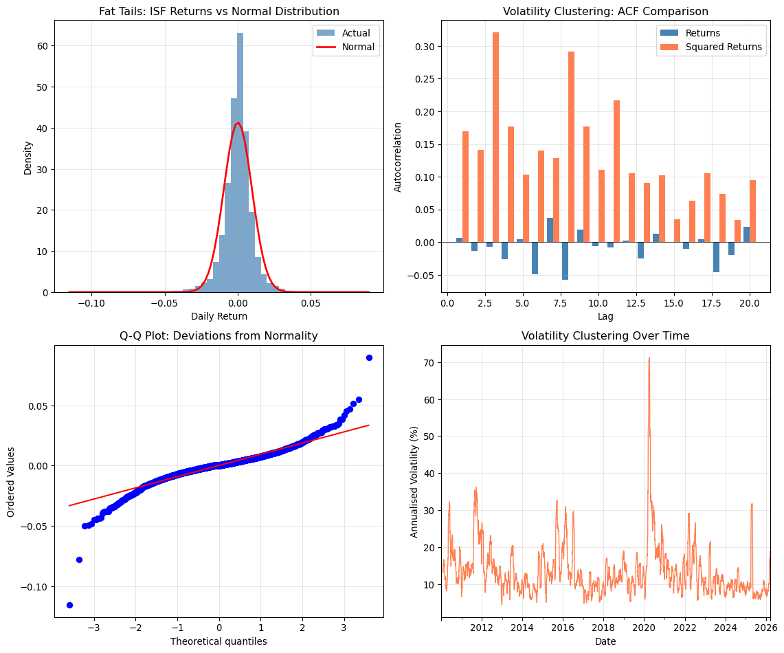
## Stylised Facts of Financial Returns
Before exploring any financial dataset, you should know what patterns to expect. The **stylised facts** of asset returns are empirical regularities observed across markets, time periods, and asset classes:
### 1. Returns Are Approximately Unpredictable
Daily returns show little autocorrelation : past returns have minimal predictive power for future returns. This is consistent with (weak) market efficiency and has profound implications for trading strategies that rely solely on historical price patterns. The autocorrelation coefficients for raw returns are typically close to zero at all lags, which is why simple momentum rules based on recent returns often fail to generate consistent profits after transaction costs.
### 2. Volatility Is Predictable and Persistent
While returns are hard to predict, squared returns (a proxy for variance) are highly autocorrelated. High volatility tends to follow high volatility : this is **volatility clustering**. This predictability is one of the best-documented stylised facts in finance and motivates the entire family of GARCH models. Practically, this means that periods of market turbulence tend to persist, which has important implications for risk management and option pricing. The volatility today contains information about the likely volatility tomorrow, even though today's return tells us little about tomorrow's return.
### 3. Returns Have Fat Tails
The distribution of returns has more extreme observations than a normal distribution would predict. The kurtosis is typically 5-10 for daily returns (compared to 3 for a normal distribution, or 0 for excess kurtosis). This means that extreme events : both positive and negative : occur far more frequently than the normal distribution suggests. Value-at-Risk (VaR) models that assume normality will systematically underestimate tail risk, which is precisely why they failed so dramatically during the 2008 financial crisis. Fat tails are not an inconvenient statistical detail; they are a fundamental feature of financial markets that risk models must address.
### 4. Returns Are Negatively Skewed
Large negative returns are more common than large positive returns of the same magnitude. Markets crash more often than they "melt up." This negative skewness reflects the asymmetry in how investors respond to good and bad news: panic selling can occur suddenly and forcefully, while optimism typically builds more gradually. The practical consequence is that downside risk is greater than simple volatility measures suggest, and portfolio insurance strategies must account for this asymmetry.
### 5. The Leverage Effect
Negative returns tend to increase subsequent volatility more than positive returns of the same size. This asymmetry is called the leverage effect, originally explained by the observation that falling stock prices increase a firm's debt-to-equity ratio, making the firm riskier and thus more volatile. More modern explanations focus on risk aversion: when markets fall, investors become more risk-averse and volatility increases. Whatever the mechanism, the practical implication is that risk increases precisely when portfolios are losing value : a particularly unhelpful property from a risk management perspective.
@tsay2010analysis summarises these patterns:
> "1. Asset returns show little serial correlations.
> 2. Asset returns are not independent. Dependence is in the squared returns.
> 3. Asset returns often show volatility clustering.
> 4. Asset returns tend to be leptokurtic (or fat-tailed).
> 5. Extreme returns appear in clusters."
These stylised facts have profound implications for modelling. Simple linear models assuming i.i.d. normal errors will be misspecified; volatility models (the GARCH family) are essential for capturing time-varying risk; risk management must account for fat tails, since VaR based on normal assumptions will underestimate tail risk; and the leverage effect means risk increases precisely when portfolios are losing value.
```{python}
#| label: stylised-facts-demo
#| fig-cap: "Stylised facts of financial returns using Bloomberg data"
import pandas as pd
import numpy as np
import matplotlib.pyplot as plt
from scipy import stats

# Load Bloomberg data (long format)
try:
    df = load_bloomberg()

    # Filter to equity data and get first available ticker
    equity_data = df[df['asset_type'] == 'Equity'].copy()

    if len(equity_data) > 0:
        # Get the first ticker with substantial data
        ticker = equity_data['ticker'].value_counts().index[0]
        ticker_data = equity_data[equity_data['ticker'] == ticker].copy()

        # Use pre-calculated returns if available, otherwise calculate from prices
        if 'return' in ticker_data.columns:
            returns = ticker_data.set_index('date')['return'].dropna()
        else:
            ticker_data = ticker_data.set_index('date')
            returns = ticker_data['PX_LAST'].pct_change().dropna()

        fig, axes = plt.subplots(2, 2, figsize=(12, 10))

        # 1. Return distribution vs normal
        ax1 = axes[0, 0]
        ax1.hist(returns, bins=50, density=True, alpha=0.7, color='steelblue', label='Actual')
        x = np.linspace(returns.min(), returns.max(), 100)
        ax1.plot(x, stats.norm.pdf(x, returns.mean(), returns.std()),
                 'r-', lw=2, label='Normal')
        ax1.set_xlabel('Daily Return')
        ax1.set_ylabel('Density')
        ax1.set_title(f'Fat Tails: {ticker} Returns vs Normal Distribution')
        ax1.legend()
        ax1.grid(alpha=0.3)

        # 2. ACF of returns vs squared returns
        ax2 = axes[0, 1]
        lags = 20
        acf_ret = [returns.autocorr(lag=i) for i in range(1, lags+1)]
        acf_sq = [(returns**2).autocorr(lag=i) for i in range(1, lags+1)]
        ax2.bar(np.arange(1, lags+1)-0.2, acf_ret, width=0.4, label='Returns', color='steelblue')
        ax2.bar(np.arange(1, lags+1)+0.2, acf_sq, width=0.4, label='Squared Returns', color='coral')
        ax2.axhline(y=0, color='k', linestyle='-', lw=0.5)
        ax2.set_xlabel('Lag')
        ax2.set_ylabel('Autocorrelation')
        ax2.set_title('Volatility Clustering: ACF Comparison')
        ax2.legend()
        ax2.grid(alpha=0.3)

        # 3. Q-Q plot
        ax3 = axes[1, 0]
        stats.probplot(returns, dist="norm", plot=ax3)
        ax3.set_title('Q-Q Plot: Deviations from Normality')
        ax3.grid(alpha=0.3)

        # 4. Rolling volatility
        ax4 = axes[1, 1]
        rolling_vol = returns.rolling(21).std() * np.sqrt(252) * 100
        rolling_vol.plot(ax=ax4, color='coral', lw=1)
        ax4.set_xlabel('Date')
        ax4.set_ylabel('Annualised Volatility (%)')
        ax4.set_title('Volatility Clustering Over Time')
        ax4.grid(alpha=0.3)

        plt.tight_layout()
        plt.show()

        # Print summary statistics
        print(f"\nSummary Statistics ({ticker}):")
        print(f"  Mean daily return: {returns.mean()*100:.3f}%")
        print(f"  Std deviation: {returns.std()*100:.3f}%")
        print(f"  Skewness: {returns.skew():.3f} (normal = 0)")
        print(f"  Kurtosis: {returns.kurtosis():.3f} (normal = 0, excess)")
        print(f"  Min return: {returns.min()*100:.2f}%")
        print(f"  Max return: {returns.max()*100:.2f}%")
    else:
        print("No equity data found in Bloomberg database.")
except FileNotFoundError:
    print("Bloomberg data not available. Run data acquisition scripts first.")
```
## Graphical Methods for Financial Data
Different plots reveal different aspects of your data:
| Plot Type | What It Reveals | Look For |
|-----------|-----------------|----------|
| **Time series plot** | Evolution over time | Trends, breaks, clustering |
| **Histogram** | Distribution shape | Fat tails, skewness, modes |
| **Q-Q plot** | Departures from reference | Heavy tails (curved ends) |
| **ACF plot** | Serial dependence | Significant lags, decay pattern |
| **Scatter plot** | Bivariate relationships | Correlations, non-linearities, outliers |
::: {.callout-tip}
## Gelman's Advice
"The relevance of this example is that we were better able to understand the data by plotting them in different ways."
:::
# Part IV: Data Quality and Validation
## Common Data Quality Issues
Financial data, even from reputable sources, can contain errors. **Price errors** include decimal point mistakes (e.g. a price of 10 recorded as 100), stale prices that are unchanged for many days, and missing splits or dividends in adjusted price series. **Volume errors** show up as zero volume on days when the market was open, or as extremely large volume spikes that may be data errors rather than genuine block trades. **Timing errors** arise from incorrect timestamps, non-monotonic date sequences, or prices incorrectly recorded on weekends or holidays. **Corporate action errors** occur when adjustment factors are missing or wrong, or when announcement and effective dates are mismatched. Any of these can distort returns, volatility estimates, and backtests, so systematic validation is essential before analysis.
## A Data Validation Framework
Before any analysis, implement systematic quality checks:
```{python}
#| label: validation-framework
#| eval: true
import pandas as pd
import numpy as np

class FinancialDataValidator:
    """
    Systematic data quality validation for financial time series.
    """

    def __init__(self, data: pd.DataFrame):
        self.data = data
        self.issues = []

    def check_timestamps(self):
        """Verify timestamp integrity."""
        if not self.data.index.is_monotonic_increasing:
            self.issues.append("FAIL: Timestamps not monotonically increasing")
        else:
            self.issues.append("PASS: Timestamp order valid")

        # Check for duplicates
        n_duplicates = self.data.index.duplicated().sum()
        if n_duplicates > 0:
            self.issues.append(f"WARN: {n_duplicates} duplicate timestamps")
        else:
            self.issues.append("PASS: No duplicate timestamps")

    def check_missing_values(self, threshold: float = 0.05):
        """Check for excessive missing values."""
        missing_pct = self.data.isnull().mean()

        for col in missing_pct.index:
            pct = missing_pct[col]
            if pct > threshold:
                self.issues.append(f"WARN: {col} has {pct:.1%} missing values")
            elif pct > 0:
                self.issues.append(f"INFO: {col} has {pct:.1%} missing values")

    def check_price_consistency(self):
        """Verify OHLC relationships."""
        if all(col in self.data.columns for col in ['Open', 'High', 'Low', 'Close']):
            # High >= Low
            invalid_hl = (self.data['High'] < self.data['Low']).sum()
            if invalid_hl > 0:
                self.issues.append(f"FAIL: {invalid_hl} days with High < Low")
            else:
                self.issues.append("PASS: High >= Low for all days")

            # Close within High-Low range
            invalid_close = ((self.data['Close'] > self.data['High']) |
                           (self.data['Close'] < self.data['Low'])).sum()
            if invalid_close > 0:
                self.issues.append(f"FAIL: {invalid_close} days with Close outside range")

    def check_extreme_returns(self, threshold: float = 0.25):
        """Flag extreme daily moves."""
        if 'Close' in self.data.columns:
            returns = self.data['Close'].pct_change()
            extreme = (returns.abs() > threshold).sum()
            if extreme > 0:
                self.issues.append(f"WARN: {extreme} extreme returns (>{threshold:.0%})")
                # Show the dates
                extreme_dates = returns[returns.abs() > threshold].index
                for d in extreme_dates[:3]:
                    self.issues.append(f"  -> {d.strftime('%Y-%m-%d')}: {returns.loc[d]:.1%}")

    def run_all_checks(self):
        """Run complete validation suite."""
        self.check_timestamps()
        self.check_missing_values()
        self.check_price_consistency()
        self.check_extreme_returns()
        return self.issues

# Demonstrate with Bloomberg data
try:
    df = load_bloomberg()
    equity_data = df[df['asset_type'] == 'Equity'].copy()

    if len(equity_data) > 0:
        # Get first ticker and create OHLC-style data for validation
        first_ticker = equity_data['ticker'].value_counts().index[0]
        ticker_data = equity_data[equity_data['ticker'] == first_ticker].copy()

        # Create sample data with required columns
        sample_data = ticker_data.set_index('date')[['PX_LAST']].copy()
        sample_data.columns = ['Close']

        validator = FinancialDataValidator(sample_data)
        results = validator.run_all_checks()

        print(f"Data Validation Report: {first_ticker}")
        print("=" * 50)
        for issue in results:
            print(f"  {issue}")
    else:
        print("No equity data found in Bloomberg database.")
except FileNotFoundError:
    print("Run Bloomberg data acquisition first.")
```
## The Missing Data Problem
Missing data in finance often follows patterns that affect analysis:
| Pattern | Description | Consequence |
|---------|-------------|-------------|
| **MCAR** | Missing Completely At Random | Unbiased (reduces power only) |
| **MAR** | Missing At Random (conditional on observed data) | Bias correctable with appropriate methods |
| **MNAR** | Missing Not At Random | Potentially serious bias |
In finance, MNAR is common: hedge funds stop reporting when performance is poor, firms delay reporting bad news, and trading halts occur during stress : precisely when data is most valuable.
### Handling Outliers: Genuine Events vs Errors
Outliers in financial data present a dilemma: they may represent genuine extreme events (which are informationally valuable) or data errors (which should be removed). The distinction matters enormously. Signs of data errors include returns that violate economic constraints (e.g. more than 100% daily loss for a stock), isolated spikes that reverse immediately, values inconsistent across data sources, and round numbers that suggest placeholder values. Signs of genuine extreme events include contemporaneous news explaining the move, consistency across related securities, persistence (the move doesn't immediately reverse), and elevated volume accompanying the price move.
**Strategies:**
| Approach | When to Use | Risk |
|----------|-------------|------|
| **Remove** | Clear data errors | Lose genuine extremes |
| **Winsorise** | Reduce influence without removing | Arbitrary threshold |
| **Robust methods** | Downweight extremes automatically | May miss tail patterns |
| **Keep all** | Studying tail behaviour | Errors contaminate analysis |
::: {.callout-warning}
## The Danger of Over-Cleaning
Aggressively removing "outliers" from financial data can eliminate precisely the observations that matter most for risk management. The 2008 financial crisis, the 2010 flash crash, and the March 2020 COVID crash were all "outliers" : and all were real.
:::
# Part V: From Raw Data to Analysis-Ready Data
## The Data Pipeline Philosophy
Production financial analysis separates **data acquisition** from **data analysis**. The acquisition stage fetches data from sources, validates it, and stores it locally; the processing stage cleans, aligns, and transforms the raw data; and the analysis stage models, visualises, and interprets the prepared data. This separation ensures reproducibility (you can re-run analysis without re-fetching data), respects rate limits (you don't hammer APIs repeatedly), and maintains temporal integrity (you know exactly when data was acquired and what was available at that time).
```{python}
#| label: data-pipeline
#| eval: true
def load_analysis_ready_data():
    """
    Load pre-processed Bloomberg data for analysis.

    This function demonstrates the production pattern:
    - Data has already been acquired and validated
    - We load cached data (fast, reproducible)
    - Analysis code doesn't need API access
    """
    try:
        df = load_bloomberg()
    except FileNotFoundError:
        print("Data not available. Run acquisition scripts first.")
        return None

    # Pivot to wide format (tickers as columns)
    prices = df.pivot_table(index='date', columns='ticker', values='PX_LAST')

    # Calculate returns
    returns = prices.pct_change().dropna()

    print("Loaded analysis-ready data:")
    print(f"  Securities: {len(prices.columns)}")
    print(f"  Date range: {prices.index[0].strftime('%Y-%m-%d')} to {prices.index[-1].strftime('%Y-%m-%d')}")
    print(f"  Observations: {len(prices)}")
    print(f"  Asset types: {df['asset_type'].unique()}")

    return {
        'prices': prices,
        'returns': returns,
        'metadata': {
            'source': 'Bloomberg Terminal',
            'last_updated': pd.Timestamp.now(),
            'raw_data': df
        }
    }

# Load data
analysis_data = load_analysis_ready_data()
```
## Documenting Data Decisions
Every analysis should document its data sources (where did each variable come from?), time period (what dates are covered and why?), universe selection (which securities are included and why?), adjustments (how were corporate actions handled?), missing data treatment (how were gaps filled or not?), and outlier treatment (were any observations removed or winsorised?). This documentation is not bureaucratic overhead : it's essential for reproducibility, peer review, and your own sanity when revisiting analysis months later. A future collaborator (or your future self) should be able to understand exactly what data was used and how it was prepared without having to reverse-engineer your code.
## A Practical Checklist
Before beginning any analysis, work through this checklist:
```{python}
#| label: data-checklist
#| eval: false
"""
Data Quality Checklist for Financial Analysis
=============================================

Run through these questions before any analysis:
"""

# 1. SOURCE AND PROVENANCE
# - Where did this data come from?
# - What is the original source (exchange, vendor, company filings)?
# - How was it processed before reaching me?
# - What is the update frequency and lag?

# 2. COVERAGE AND SELECTION
# - What universe does this cover?
# - What is excluded and why?
# - Is there survivorship bias?
# - How are corporate actions handled?

# 3. TEMPORAL INTEGRITY
# - What timezone are timestamps in?
# - Are there gaps (weekends, holidays, halts)?
# - Is this point-in-time or restated data?
# - What is the effective date vs announcement date?

# 4. MEASUREMENT QUALITY
# - What does each variable actually measure?
# - What are the units and scaling?
# - How are missing values coded?
# - What is the precision/rounding?

# 5. KNOWN ISSUES
# - Are there documented data quality issues?
# - Have there been methodology changes over time?
# - Are there known outliers or special situations?

# 6. VALIDATION PERFORMED
# - Basic statistics computed and reviewed?
# - Distributions examined for anomalies?
# - Cross-checked against alternative sources?
# - Time series plotted and inspected?
```
# Summary and Key Takeaways
## The Data Mindset
The core principles of rigorous data practice in finance can be summarised as follows: question everything about where your numbers come from and what assumptions are embedded in them; recognise that selection bias is everywhere (survivorship, availability, reporting : be paranoid about what's missing); remember that proxies are imperfect and the gap between measurement and construct is often larger than we'd like; look before you model, since exploratory analysis reveals problems that no amount of sophisticated modelling can fix; and validate systematically by automating quality checks so they run every time. These principles distinguish rigorous analysis from "plug-and-play" statistics, and they separate research that produces reliable insights from research that produces spurious patterns.
## Connecting to What's Next
This chapter establishes the **data foundations** that support everything else in the course. The foundations chapter assumes your data is appropriate for the questions you're asking; the volatility chapter assumes your data exhibits the stylised facts we've discussed; and the machine learning chapters rest on the principle that garbage in means garbage out : data quality determines model quality.
## Exercises
### Conceptual Questions
1. **DGP Analysis**: Choose a financial dataset you work with regularly. Write a one-page description of its data generating process, including: (a) the original source, (b) how it was collected, (c) what selection rules determine inclusion, and (d) what transformations have been applied.
2. **Selection Bias**: A researcher reports that hedge funds in their database earned 12% annually over the past decade. What forms of selection bias might affect this estimate? How would you expect the true average hedge fund return to compare?
3. **Validity vs Reliability**: For each of the following, discuss whether the main concern is validity, reliability, or both:
- Using analyst earnings forecasts to measure market expectations
- Using daily closing prices to measure intraday volatility
- Using credit ratings to measure default probability
### Practical Exercises
4. **EDA Practice**: Using the Bloomberg database (or another source), conduct a complete exploratory analysis of a single stock's returns:
- Compute summary statistics and compare to stylised facts
- Create the four-panel diagnostic plot (histogram, ACF, Q-Q, rolling volatility)
- Identify any outliers and investigate whether they are genuine or errors
5. **Validation Implementation**: Extend the `FinancialDataValidator` class to include:
- A check for stale prices (unchanged for >5 consecutive days)
- A check for weekend/holiday data points
- A check for negative prices or volumes
6. **Survivorship Bias Simulation**: Modify the survivorship bias simulation to explore:
- How does the bias change with different failure thresholds?
- What if funds with extreme positive returns also close (to lock in gains)?
- How does the bias evolve over different time horizons?
---
## Further Reading
For deeper exploration of these topics:
- @gelman2020regression Chapter 2 ("Data and Measurement") : the philosophical foundations
- @tsay2010analysis Chapter 1 ("Financial Time Series and Their Characteristics") : stylised facts
- @brooks2019introductory Chapter 1 ("Introduction") : data types in finance
- @deprado2018advances Chapters 2-3 ("Financial Data Structures" and "Labeling") : modern data engineering
---
## References
::: {#refs}
:::