Show code
try:
    import yfinance, pandas, pandas_datareader
except Exception:
!pip -q install yfinance pandas pandas-datareaderBuild a Reliable Pipeline with Free APIs (Colab Version)
This is the Colab version using free APIs (yfinance). For the in-class Bloomberg Terminal session (Excel add-in), see Lab 2: Survivorship Bias in UK Banking.
Expected Time:
![]()
Ulster students have access to ~20 Bloomberg terminals in the Financial Innovation Lab. The in-class Week 2 lab uses the Bloomberg Excel add-in to quantify survivorship bias with UK banking crisis data: Lab 2: Survivorship Bias in UK Banking.
try:
import yfinance, pandas, pandas_datareader
except Exception:
!pip -q install yfinance pandas pandas-datareaderReal-world financial data science starts with data acquisition. APIs are your gateway to market data, but they’re unreliable: rate limits, outages, data quality issues. Professional systems need resilience: retry logic, fallback sources, validation, and logging.
1. Resilience → Handle API failures gracefully (retries, fallbacks, synthetic data)
2. Validation → Check data quality before analysis (missing values, outliers, gaps)
3. Provenance → Log data sources and transformations (reproducibility, debugging)
These aren’t optional extras: they’re the difference between research toys and production systems.
By the end of this lab, you will have:
Time estimate: ≈ 60 minutes (plus optional extensions)
In projects and assessments, you’ll often build models (or trading rules) on top of a data pipeline. If your pipeline has silent bugs (wrong dates, missing values, look-ahead bias), your entire analysis is invalidated. Build good habits now.
This task implements a resilient data pipeline: try yfinance first, fall back to Stooq if it fails, use synthetic data as last resort. This three-tier approach ensures your analysis never stops due to API failures.
Why we need fallbacks: - Free APIs have rate limits (yfinance: ~2000 calls/hour) - APIs go down (maintenance, outages, deprecated endpoints) - Network issues are common in cloud environments
Three-tier strategy: 1. Primary: yfinance (best for US equities, free, widely used) 2. Fallback: Stooq via pandas-datareader (alternative free source) 3. Last resort: Synthetic data (ensures code always runs for testing)
This pattern appears in production systems at every scale.
import os, time, random
import yfinance as yf
import pandas as pd
import numpy as np

symbols = ['AAPL', 'MSFT', 'SPY']

def get_close_from_yf(symbols, period='2y', tries=3):
    """
    Fetch adjusted closing prices from Yahoo Finance with retry logic.

    Implements exponential backoff to handle rate limits gracefully. Returns
    adjusted prices (splits/dividends applied) suitable for return calculations.

    Parameters
    ----------
    symbols : list of str
        Stock tickers (e.g., ['AAPL', 'MSFT'])
    period : str, default='2y'
        Data period: '1d', '5d', '1mo', '3mo', '6mo', '1y', '2y', '5y', '10y', 'ytd', 'max'
    tries : int, default=3
        Number of retry attempts before raising error

    Returns
    -------
    pd.DataFrame
        Adjusted closing prices with DatetimeIndex and symbol columns

    Raises
    ------
    RuntimeError
        If all retry attempts fail

    Notes
    -----
    - Uses `auto_adjust=True` to get split/dividend-adjusted prices
    - Implements exponential backoff: waits 2, 4, 6 seconds between retries
    - Handles yfinance MultiIndex columns (multiple symbols) vs single-symbol format
    - Returns empty rows are filtered (only keeps days with at least one price)

    Examples
    --------
    >>> prices = get_close_from_yf(['AAPL', 'MSFT'], period='1y')
    >>> prices.shape
    (252, 2)  # Roughly 252 trading days in a year
    >>> prices.iloc[-1]  # Most recent closing prices
    AAPL    182.50
    MSFT    415.20
    """
    last_err = None

    for attempt in range(tries):
        try:
            # Download with adjusted prices (splits/dividends applied)
            df = yf.download(symbols, period=period, auto_adjust=True,
                           progress=False, group_by='ticker', threads=True)

            # yfinance returns MultiIndex columns when fetching multiple symbols
            if isinstance(df.columns, pd.MultiIndex):
                # Extract 'Close' price for each symbol
                closes = pd.concat(
                    {sym: df[sym]['Close'] for sym in symbols if sym in df.columns.levels[0]},
                    axis=1
                )
                closes.columns = [c if isinstance(c, str) else c[0] for c in closes.columns]
            else:
                # Single symbol returns simple columns
                closes = df['Close'].to_frame(symbols[0])

            # Only return if we got at least one non-empty row
            if closes.dropna(how='all').shape[0] > 0:
                return closes

        except Exception as e:
            last_err = e

        # Exponential backoff with jitter to avoid thundering herd
        time.sleep(2 * (attempt + 1) + random.random())

    raise RuntimeError(f"yfinance download failed after {tries} tries: {last_err}")


def get_close_from_stooq(symbols, years=2):
    """
    Fetch closing prices from Stooq via pandas-datareader (fallback source).

    Stooq provides historical price data for global markets. This function
    serves as fallback when yfinance fails. Fetches data sequentially to
    respect rate limits.

    Parameters
    ----------
    symbols : list of str
        Stock tickers (e.g., ['AAPL', 'MSFT'])
    years : int, default=2
        Number of years of historical data to fetch

    Returns
    -------
    pd.DataFrame
        Closing prices with DatetimeIndex (sorted) and symbol columns

    Raises
    ------
    RuntimeError
        If no symbols successfully fetched

    Notes
    -----
    - Fetches symbols sequentially (not parallel) to respect rate limits
    - Waits 0.4 seconds between requests
    - Silently skips symbols that fail (rather than stopping entire process)
    - Returns only successfully fetched symbols

    Examples
    --------
    >>> prices = get_close_from_stooq(['AAPL'], years=1)
    >>> prices.index.name
    'Date'
    """
    from datetime import datetime, timedelta
    from pandas_datareader import data as web

    # Define date range
    end = datetime.today()
    start = end - timedelta(days=365 * years + 14)  # Extra days for weekends/holidays

    series = []
    for sym in symbols:
        try:
            # Fetch from Stooq and extract 'Close' column
            s = web.DataReader(sym, 'stooq', start, end)['Close'].sort_index()
            s.name = sym
            series.append(s)

            # Respectful rate limiting
            time.sleep(0.4)
        except Exception:
            # Skip symbols that fail rather than stopping entire fetch
            pass

    if not series:
        raise RuntimeError("stooq fallback returned no data")

    return pd.concat(series, axis=1)


def synthetic_prices(symbols, periods=252, mu=0.0004, sigma=0.012):
    """
    Generate synthetic price series using geometric Brownian motion.

    This is a last-resort fallback when all real APIs fail. Useful for
    testing and development when APIs are unavailable. NOT FOR ANALYSIS.

    Parameters
    ----------
    symbols : list of str
        Symbol names for columns (can be anything)
    periods : int, default=252
        Number of business days to generate (~1 year of trading days)
    mu : float, default=0.0004
        Daily drift (mean return): 0.0004 ≈ 10% annual
    sigma : float, default=0.012
        Daily volatility: 0.012 ≈ 19% annual volatility

    Returns
    -------
    pd.DataFrame
        Synthetic prices starting at 100, with business day index

    Notes
    -----
    - Uses fixed seed (42) for reproducibility
    - Generates prices via: P(t) = 100 * exp(cumsum(returns))
    - Returns ~ Normal(mu, sigma) independently across symbols
    - Index: business days ending at today

    Examples
    --------
    >>> synth = synthetic_prices(['SYN1', 'SYN2'], periods=10)
    >>> synth.shape
    (10, 2)
    >>> (synth.iloc[-1] / synth.iloc[0]).mean()  # Typical growth
    1.04  # Roughly 4% over 10 days

    Warnings
    --------
    DO NOT use for actual analysis. This is for code testing only.
    """
    rng = np.random.default_rng(42)  # Fixed seed for reproducibility

    # Business day index ending today
    dates = pd.bdate_range(end=pd.Timestamp.today().normalize(), periods=periods)

    # Generate returns: Normal(mu, sigma)
    shocks = rng.normal(mu, sigma, size=(len(dates), len(symbols)))

    # Convert to prices: P(t) = P(0) * exp(cumsum(returns))
    levels = 100 * np.exp(np.cumsum(shocks, axis=0))

return pd.DataFrame(levels, index=dates, columns=symbols)# === Try primary source (yfinance) ===
try:
prices = get_close_from_yf(symbols)
source = 'yfinance'
print(f"✔ Successfully fetched from yfinance")
except Exception as e1:
print(f"⚠ yfinance failed: {e1}")
# === Try fallback source (Stooq) ===
try:
prices = get_close_from_stooq(symbols)
source = 'stooq (pandas-datareader)'
print(f"✔ Successfully fetched from Stooq fallback")
except Exception as e2:
print(f"⚠ Stooq failed: {e2}")
# === Last resort: synthetic data ===
prices = synthetic_prices(symbols)
source = f'synthetic (fallback due to API failures)'
print(f"⚠ Using synthetic data (NOT for real analysis!)")
# Display first and last few rows
print(f"\nData shape: {prices.shape}")
print(f"\nFirst 3 rows:")
print(prices.head(3))
print(f"\nLast 3 rows:")
print(prices.tail(3))⚠ yfinance failed: yfinance download failed after 3 tries: None
✔ Successfully fetched from Stooq fallback
Data shape: (511, 3)
First 3 rows:
AAPL MSFT SPY
Date
2024-02-28 179.953 405.442 498.350
2024-02-29 179.286 411.329 500.142
2024-03-01 178.207 413.179 504.838
Last 3 rows:
AAPL MSFT SPY
Date
2026-03-10 260.72 405.76 677.18
2026-03-11 260.81 404.88 676.33
2026-03-12 255.76 401.86 666.06The try-except cascade ensures you always get data, even if APIs fail. In production, you’d add alerts when fallbacks activate so engineers can investigate the primary failure.
# === Build provenance log ===
log = {}
log['source'] = source
log['symbols_requested'] = len(symbols)
log['symbols_received'] = len(prices.columns)
log['date_range'] = f"{prices.index[0]} to {prices.index[-1]}"
log['trading_days'] = len(prices)

# === Check for missing prices ===
log['missing_prices'] = int(prices.isna().sum().sum())
log['missing_pct'] = f"{(prices.isna().sum().sum() / prices.size * 100):.2f}%"

# === Calculate returns and check quality ===
rets = prices.pct_change()
log['missing_returns'] = int(rets.isna().sum().sum())

# === Flag outliers (|return| > 20% = likely data error or halt) ===
log['out_of_range'] = int((rets.abs() > 0.2).sum().sum())

# Display log
import json
print("\n=== Data Quality Log ===")
print(json.dumps(log, indent=2))

# === Quality gate ===
if prices.dropna(how='all').shape[0] > 0:
    print(f"\n✔ Data source: {source}")
    print(f"✔ Download and validation checks passed")
else:
    print(f"\n⚠ Warning: no data returned from any source")
=== Data Quality Log ===
{
  "source": "stooq (pandas-datareader)",
  "symbols_requested": 3,
  "symbols_received": 3,
  "date_range": "2024-02-28 00:00:00 to 2026-03-12 00:00:00",
  "trading_days": 511,
  "missing_prices": 0,
  "missing_pct": "0.00%",
  "missing_returns": 3,
  "out_of_range": 0
}

✔ Data source: stooq (pandas-datareader)
✔ Download and validation checks passedRule of thumb: <1% missing is acceptable, >5% requires investigation
Checkpoint: Look at your log. Which quality issues did you find? How would you handle them differently for a production system vs. academic analysis?
Raw data always has issues. Professional practice: clean conservatively and document decisions.
# === Remove rows where all returns are missing ===
clean = rets.dropna()

print(f"Original shape: {rets.shape}")
print(f"After dropna: {clean.shape}")
print(f"Rows removed: {rets.shape[0] - clean.shape[0]}")

# === Clip extreme values (conservative approach) ===
# Instead of deleting outliers, cap them at reasonable limits
# -20% to +20% captures 99%+ of normal daily returns
clean_clipped = clean.clip(lower=-0.2, upper=0.2)

# Count how many values were clipped
clipped_low = (clean < -0.2).sum().sum()
clipped_high = (clean > 0.2).sum().sum()

print(f"\n=== Outlier Treatment ===")
print(f"Values clipped at lower bound (-20%): {clipped_low}")
print(f"Values clipped at upper bound (+20%): {clipped_high}")

# Display sample
print(f"\nCleaned returns (last 5 days):")
print(clean_clipped.tail())
Original shape: (511, 3)
After dropna: (510, 3)
Rows removed: 1
=== Outlier Treatment ===
Values clipped at lower bound (-20%): 0
Values clipped at upper bound (+20%): 0
Cleaned returns (last 5 days):
AAPL MSFT SPY
Date
2026-03-06 -0.010720 -0.004992 -0.013107
2026-03-09 0.009438 0.001762 0.008760
2026-03-10 0.003194 -0.008770 -0.001607
2026-03-11 0.000345 -0.002169 -0.001255
2026-03-12 -0.019363 -0.007459 -0.015185# === Save to CSV for later use ===
clean_clipped.to_csv('returns_clean.csv')
# === Verify file was created ===
import os
if os.path.exists('returns_clean.csv'):
file_size = os.path.getsize('returns_clean.csv')
print(f"✔ Saved returns_clean.csv ({file_size:,} bytes)")
else:
print("⚠ Warning: File not created")
# === Document the cleaning process ===
cleaning_log = {
'rows_original': rets.shape[0],
'rows_after_dropna': clean.shape[0],
'values_clipped_low': int(clipped_low),
'values_clipped_high': int(clipped_high),
'clip_bounds': '[-20%, +20%]',
'output_file': 'returns_clean.csv'
}
print(f"\n=== Cleaning Summary ===")
print(json.dumps(cleaning_log, indent=2))✔ Saved returns_clean.csv (38,609 bytes)
=== Cleaning Summary ===
{
"rows_original": 511,
"rows_after_dropna": 510,
"values_clipped_low": 0,
"values_clipped_high": 0,
"clip_bounds": "[-20%, +20%]",
"output_file": "returns_clean.csv"
}Deliverable: Write a short note (100-150 words) describing: - What issues you found (missing values, outliers) - How you handled them (dropna, clipping) - Why these choices are appropriate for financial return data - What trade-offs you made (e.g., information loss vs. robustness)
auto_adjust=True.This short exercise previews a factor dataset (JKP). Load a small sample CSV, compute quick stats, and (optionally) run a one‑line CAPM alpha.
# JKP sample (course mirror) :  small monthly slice with MKT, SMB, HML, MOM
import pandas as pd, os
import statsmodels.api as sm

# Prefer local file during site build; fall back to raw GitHub if needed
local_path = os.path.join('..','resources','jkp-sample.csv')
if os.path.exists(local_path):
    jkp = pd.read_csv(local_path, parse_dates=['date']).set_index('date').sort_index()
else:
    # Use public notebooks repo URL for Colab
    url = "https://raw.githubusercontent.com/quinfer/fin510-colab-notebooks/main/resources/jkp-sample.csv"
    jkp = pd.read_csv(url, parse_dates=['date']).set_index('date').sort_index()

# Summary stats and quick cumulative return for MOM
summary = jkp[['MKT','SMB','HML','MOM']].describe().round(3)
cum = (1 + jkp['MOM']).cumprod() - 1
summary.tail(3), cum.tail()

# Optional: CAPM alpha (no HAC here :  use HAC in the assessment)
ls = jkp['MOM'].dropna()
mkt = jkp['MKT'].reindex(ls.index)
capm = sm.OLS(ls, sm.add_constant(mkt)).fit()
float(capm.params['const']), float(capm.tvalues['const'])
(0.005408343449950338, 1.763810502676042)Notes - In the assessment you will use a larger CSV downloaded from the JKP portal and apply HAC standard errors. - Keep scope tight (few factors, limited window) and focus on quality of evidence.
# Ensure prediction tasks shift the target correctly
import pandas as pd

# Intentionally wrong design (no shift) for demonstration
X_wrong = jkp[['MKT','SMB','HML','MOM']].dropna()
y_next   = jkp['MOM'].shift(-1)               # next-month target

# Overlap of indices indicates potential leakage if you don't drop/shift properly
overlap = X_wrong.index.intersection(y_next.dropna().index)
print("Potential leakage rows with wrong design:", len(overlap))

# Correct design: predictors at t, target at t+1 → align and drop NA
X = jkp[['MKT','SMB','HML']].shift(0)
y = jkp['MOM'].shift(-1)
df = pd.concat([X, y.rename('y')], axis=1).dropna()
print("Rows after proper shift/drop:", len(df))
Potential leakage rows with wrong design: 9
Rows after proper shift/drop: 9This extension connects to the lecture material on empirical regularities in financial returns. Before analysing any financial dataset, you should verify it exhibits the known stylised facts.
Financial returns consistently show:
These are empirical facts, not assumptions. Your data should exhibit them.
from statsmodels.graphics.tsaplots import plot_acf
import matplotlib.pyplot as plt

# Use one asset from your cleaned returns
returns_series = clean_clipped.iloc[:, 0].dropna()  # First column

fig, axes = plt.subplots(1, 2, figsize=(14, 5))

# ACF of returns (should be weak)
ax1 = axes[0]
plot_acf(returns_series, lags=20, ax=ax1, alpha=0.05)
ax1.set_title('ACF: Returns (Should be Weak)')
ax1.set_xlabel('Lag (days)')

# Scatter plot: r(t) vs r(t-1)
ax2 = axes[1]
ax2.scatter(returns_series.shift(1), returns_series, alpha=0.3, s=10)
ax2.axhline(y=0, color='gray', linestyle='--', lw=1)
ax2.axvline(x=0, color='gray', linestyle='--', lw=1)
ax2.set_xlabel('Return(t-1)')
ax2.set_ylabel('Return(t)')
ax2.set_title('Returns vs Lagged Returns')
ax2.grid(alpha=0.3)

plt.tight_layout()
plt.show()

# Quantify
lag1_corr = returns_series.autocorr(lag=1)
print(f"\nLag-1 autocorrelation: {lag1_corr:.4f}")
print("Interpretation: Near zero → returns are approximately unpredictable")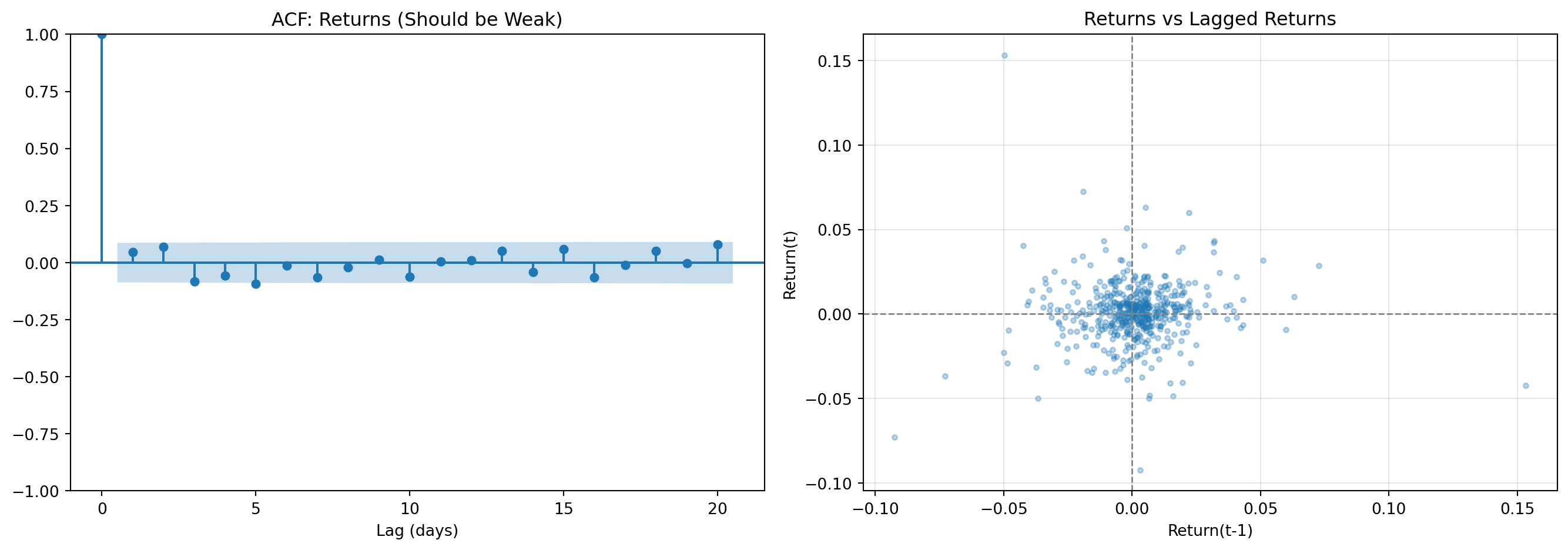
Lag-1 autocorrelation: 0.0459
Interpretation: Near zero → returns are approximately unpredictable# Compare ACF of returns vs squared returns (volatility proxy)
fig, axes = plt.subplots(1, 2, figsize=(14, 5))
ax1 = axes[0]
plot_acf(returns_series, lags=20, ax=ax1, alpha=0.05)
ax1.set_title('ACF: Returns (Weak)')
ax2 = axes[1]
plot_acf(returns_series**2, lags=20, ax=ax2, alpha=0.05)
ax2.set_title('ACF: Squared Returns (Strong = Clustering)')
plt.tight_layout()
plt.show()
# Quantify
acf_ret_lag1 = returns_series.autocorr(lag=1)
acf_sq_lag1 = (returns_series**2).autocorr(lag=1)
print(f"\nReturns ACF(1): {acf_ret_lag1:.4f}")
print(f"Squared returns ACF(1): {acf_sq_lag1:.4f}")
print("\nInterpretation: Squared returns show strong persistence → volatility clustering")
print("This is why GARCH models are needed for volatility forecasting")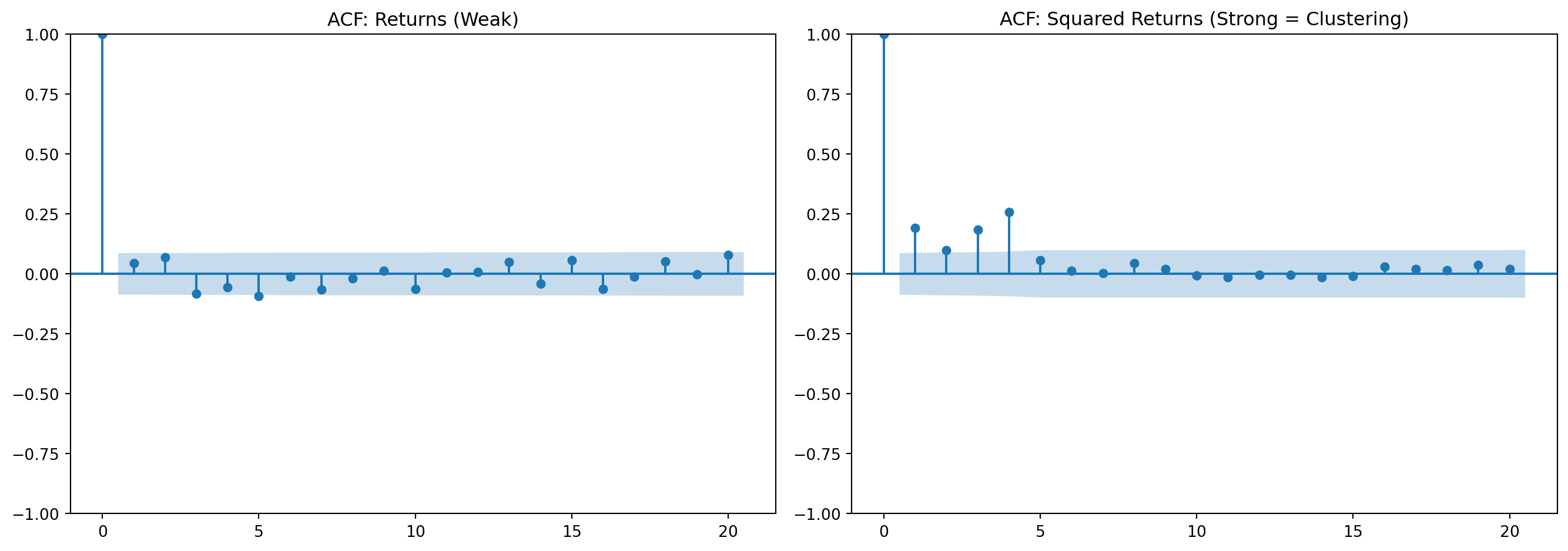
Returns ACF(1): 0.0459
Squared returns ACF(1): 0.1908

Interpretation: Squared returns show strong persistence → volatility clustering
This is why GARCH models are needed for volatility forecastingfrom scipy import stats
fig, axes = plt.subplots(1, 2, figsize=(14, 5))
# Q-Q plot (curved ends = fat tails)
ax1 = axes[0]
stats.probplot(returns_series, dist="norm", plot=ax1)
ax1.set_title('Q-Q Plot: Returns vs Normal Distribution')
ax1.grid(alpha=0.3)
# Histogram vs Normal
ax2 = axes[1]
ax2.hist(returns_series, bins=50, density=True, alpha=0.7,
color='steelblue', label='Empirical', edgecolor='black')
x = np.linspace(returns_series.min(), returns_series.max(), 100)
ax2.plot(x, stats.norm.pdf(x, returns_series.mean(), returns_series.std()),
'r-', lw=2, label='Normal')
ax2.set_xlabel('Daily Return')
ax2.set_ylabel('Density')
ax2.set_title('Distribution: Empirical vs Normal')
ax2.legend()
ax2.grid(alpha=0.3)
plt.tight_layout()
plt.show()
# Quantify
kurtosis = returns_series.kurtosis()
_, p_norm = stats.normaltest(returns_series)
print(f"\nExcess kurtosis: {kurtosis:.2f} (Normal = 0)")
print(f"Normality test p-value: {p_norm:.4f}")
if p_norm < 0.05:
print("→ Reject normality: fat tails are present")
else:
print("→ Cannot reject normality (unusual for financial data)")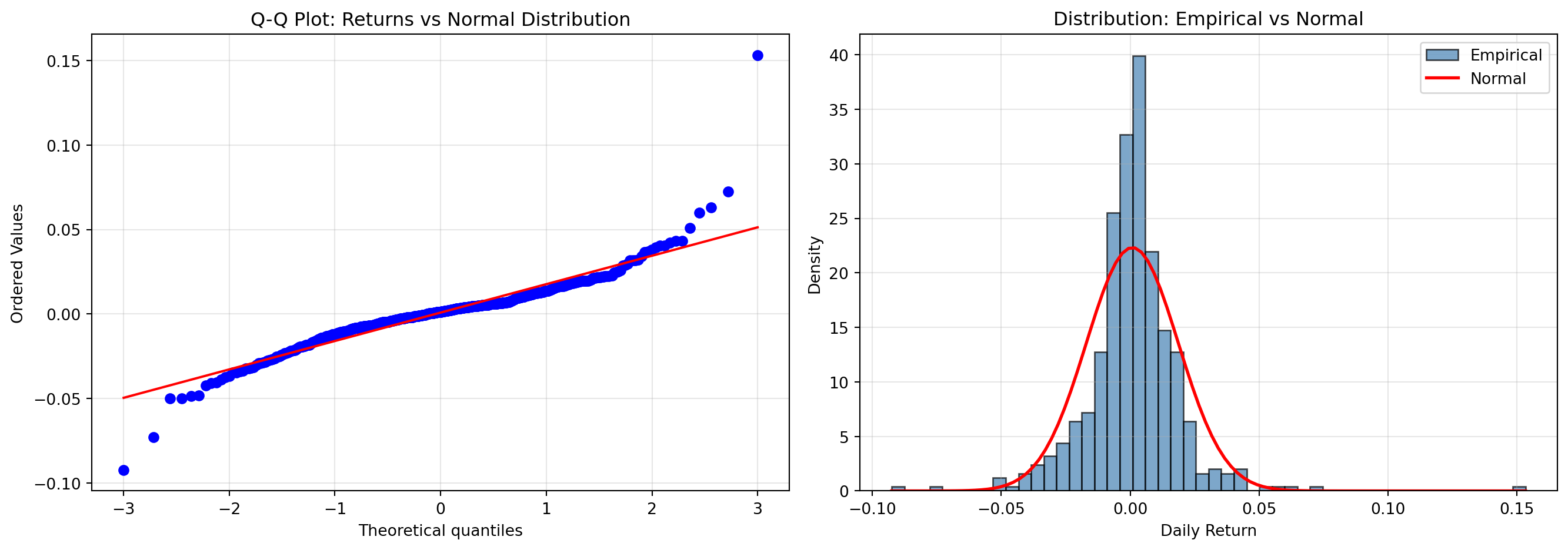
Excess kurtosis: 12.76 (Normal = 0)
Normality test p-value: 0.0000
→ Reject normality: fat tails are present# Skewness analysis
skewness = returns_series.skew()
# Compare tail quantiles
left_5pct = float(returns_series.quantile(0.05))
right_5pct = float(returns_series.quantile(0.95))
median_val = float(returns_series.median())
fig, ax = plt.subplots(figsize=(10, 6))
ax.hist(returns_series, bins=50, alpha=0.7, color='steelblue', edgecolor='black')
ax.axvline(x=left_5pct, color='red', linestyle='--', lw=2,
label=f'5th %ile: {left_5pct:.4f}')
ax.axvline(x=right_5pct, color='green', linestyle='--', lw=2,
label=f'95th %ile: {right_5pct:.4f}')
ax.axvline(x=median_val, color='gray', linestyle='-', lw=1, label='Median')
ax.set_xlabel('Daily Return')
ax.set_ylabel('Frequency')
ax.set_title('Return Distribution: Checking for Skewness')
ax.legend()
ax.grid(alpha=0.3, axis='y')
plt.tight_layout()
plt.show()
print(f"\nSkewness: {skewness:.3f}")
if skewness < 0:
print("→ Negative skewness: left tail is longer (crashes > melt-ups)")
else:
print("→ Positive skewness: right tail is longer (unusual)")
print(f"\nLeft tail (5th %ile): {left_5pct:.4f}")
print(f"Right tail (95th %ile): {right_5pct:.4f}")
print(f"Tail asymmetry: {abs(left_5pct) / abs(right_5pct):.2f}")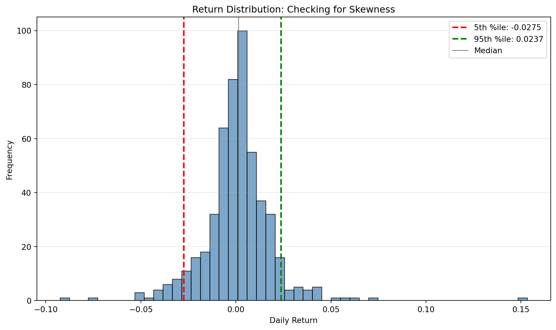
Skewness: 0.898
→ Positive skewness: right tail is longer (unusual)

Left tail (5th %ile): -0.0275
Right tail (95th %ile): 0.0237
Tail asymmetry: 1.16# Summary of all stylised facts
print("=" * 60)
print("STYLISED FACTS VERIFICATION SUMMARY")
print("=" * 60)
print(f"\n1. Return Autocorrelation (Lag 1): {acf_ret_lag1:.4f}")
if abs(acf_ret_lag1) < 0.1:
print(" ✓ PASS: Weak autocorrelation (returns unpredictable)")
else:
print(" ⚠ CHECK: Strong autocorrelation detected")
print(f"\n2. Volatility Clustering ACF (Lag 1): {acf_sq_lag1:.4f}")
if acf_sq_lag1 > 0.1:
print(" ✓ PASS: Volatility clustering present")
else:
print(" ⚠ CHECK: Weak volatility clustering")
print(f"\n3. Excess Kurtosis: {kurtosis:.2f}")
if kurtosis > 1:
print(" ✓ PASS: Fat tails present (kurtosis > 1)")
else:
print(" ⚠ CHECK: Tails may not be fat enough")
print(f"\n4. Skewness: {skewness:.3f}")
if skewness < 0:
print(" ✓ PASS: Negative skewness (crash risk > upside)")
else:
print(" ⚠ CHECK: Positive or zero skewness (unusual)")
print(f"\n5. Normality Test p-value: {p_norm:.4f}")
if p_norm < 0.05:
print(" ✓ PASS: Non-normal distribution (expected)")
else:
print(" ⚠ CHECK: Cannot reject normality (unusual for returns)")
print("\n" + "=" * 60)
print("\nIf your data passes most checks, it exhibits realistic properties.")
print("If not, investigate: data errors? wrong frequency? synthetic data?")============================================================
STYLISED FACTS VERIFICATION SUMMARY
============================================================
1. Return Autocorrelation (Lag 1): 0.0459
✓ PASS: Weak autocorrelation (returns unpredictable)
2. Volatility Clustering ACF (Lag 1): 0.1908
✓ PASS: Volatility clustering present
3. Excess Kurtosis: 12.76
✓ PASS: Fat tails present (kurtosis > 1)
4. Skewness: 0.898
⚠ CHECK: Positive or zero skewness (unusual)
5. Normality Test p-value: 0.0000
✓ PASS: Non-normal distribution (expected)
============================================================
If your data passes most checks, it exhibits realistic properties.
If not, investigate: data errors? wrong frequency? synthetic data?Write a brief note (150-200 words) answering:
Submit via Blackboard if completing for credit.
This extension directly applies concepts from:
You’ve now built a complete data pipeline with:
These patterns transfer to all financial data work : use them in every future analysis.
Next lab: Quantify survivorship bias using Bloomberg Terminal (in-class, Excel add-in) or explore alternative data sources (homework extension).